Ridge2FoldCV for data with low effective rank

In this notebook we explain in more detail how skmatter.linear_model.Ridge2FoldCV speeds up the cross-validation optimizing the regularitzation parameter :param alpha: and compare it with existing solution for that in scikit-learn slearn.linear_model.RidgeCV. skmatter.linear_model.Ridge2FoldCV was designed to predict efficiently feature matrices, but it can be also useful for the prediction single targets.

import time

import matplotlib.pyplot as plt
import numpy as np
from sklearn.datasets import make_regression
from sklearn.linear_model import RidgeCV
from sklearn.metrics import mean_squared_error
from sklearn.model_selection import KFold, train_test_split

from skmatter.linear_model import Ridge2FoldCV

SEED = 12616
N_REPEAT_MICRO_BENCH = 5

Numerical instabilities of sklearn leave-one-out CV

In linear regression, the complexity of computing the weight matrix is theoretically bounded by the inversion of the covariance matrix. This is more costly when conducting regularized regression, wherein we need to optimise the regularization parameter in a cross-validation (CV) scheme, thereby recomputing the inverse for each parameter. scikit-learn offers an efficient leave-one-out CV (LOO CV) for its ridge regression which avoids these repeated computations [loocv]. Because we needed an efficient ridge that works in predicting for the reconstruction measures in skmatter.metrics we implemented with skmatter.linear_model.Ridge2FoldCV an efficient 2-fold CV ridge regression that uses a singular value decomposition (SVD) to reuse it for all regularization parameters \(\lambda\). Assuming we have the standard regression problem optimizing the weight matrix in

\[\begin{align} \|\mathbf{X}\mathbf{W} - \mathbf{Y}\| \end{align}\]

Here \(\mathbf{Y}\) can be seen also a matrix as it is in the case of multi target learning. Then in 2-fold cross validation we would predict first the targets of fold 2 using fold 1 to estimate the weight matrix and vice versa. Using SVD the scheme estimation on fold 1 looks like this.

\[\begin{split}\begin{align} &\mathbf{X}_1 = \mathbf{U}_1\mathbf{S}_1\mathbf{V}_1^T, \qquad\qquad\qquad\quad \textrm{feature matrix }\mathbf{X}\textrm{ for fold 1} \\ &\mathbf{W}_1(\lambda) = \mathbf{V}_1 \tilde{\mathbf{S}}_1(\lambda)^{-1} \mathbf{U}_1^T \mathbf{Y}_1, \qquad \textrm{weight matrix fitted on fold 1}\\ &\tilde{\mathbf{Y}}_2 = \mathbf{X}_2 \mathbf{W}_1, \qquad\qquad\qquad\qquad \textrm{ prediction of }\mathbf{Y}\textrm{ for fold 2} \end{align}\end{split}\]

The efficient 2-fold scheme in Ridge2FoldCV reuses the matrices

\[\begin{align} &\mathbf{A}_1 = \mathbf{X}_2 \mathbf{V}_1, \quad \mathbf{B}_1 = \mathbf{U}_1^T \mathbf{Y}_1. \end{align}\]

for each fold to not recompute the SVD. The computational complexity after the initial SVD is thereby reduced to that of matrix multiplications.

We first create an artificial dataset

X, y = make_regression(
    n_samples=1000,
    n_features=400,
    random_state=SEED,
)

# regularization parameters
alphas = np.geomspace(1e-12, 1e-1, 12)

# 2 folds for train and validation split
cv = KFold(n_splits=2, shuffle=True, random_state=SEED)

skmatter_ridge_2foldcv_cutoff = Ridge2FoldCV(
    alphas=alphas, regularization_method="cutoff", cv=cv
)

skmatter_ridge_2foldcv_tikhonov = Ridge2FoldCV(
    alphas=alphas, regularization_method="tikhonov", cv=cv
)

sklearn_ridge_2foldcv_tikhonov = RidgeCV(
    alphas=alphas,
    cv=cv,
    fit_intercept=False,  # remove the incluence of learning bias
)

sklearn_ridge_loocv_tikhonov = RidgeCV(
    alphas=alphas,
    cv=None,
    fit_intercept=False,  # remove the incluence of learning bias
)

Now we do simple benchmarks

def micro_bench(ridge):
    """A small benchmark function."""
    global N_REPEAT_MICRO_BENCH, X, y
    timings = []
    train_mse = []
    test_mse = []
    for _ in range(N_REPEAT_MICRO_BENCH):
        X_train, X_test, y_train, y_test = train_test_split(
            X, y, train_size=0.5, random_state=SEED
        )
        start = time.time()
        ridge.fit(X_train, y_train)
        end = time.time()
        timings.append(end - start)
        train_mse.append(mean_squared_error(y_train, ridge.predict(X_train)))
        test_mse.append(mean_squared_error(y_test, ridge.predict(X_test)))

    print(f"  Time: {np.mean(timings)}s")
    print(f"  Train MSE: {np.mean(train_mse)}")
    print(f"  Test MSE: {np.mean(test_mse)}")


print("skmatter 2-fold CV cutoff")
micro_bench(skmatter_ridge_2foldcv_cutoff)
print()
print("skmatter 2-fold CV tikhonov")
micro_bench(skmatter_ridge_2foldcv_tikhonov)
print()
print("sklearn 2-fold CV tikhonov")
micro_bench(sklearn_ridge_2foldcv_tikhonov)
print()
print("sklearn leave-one-out CV")
micro_bench(sklearn_ridge_loocv_tikhonov)

skmatter 2-fold CV cutoff
  Time: 0.08593254089355469s
  Train MSE: 1.4179323700682082e-25
  Test MSE: 3.274563400398066e-25

skmatter 2-fold CV tikhonov
  Time: 0.08517122268676758s
  Train MSE: 0.006720047338465212
  Test MSE: 0.22910125130751807

sklearn 2-fold CV tikhonov
  Time: 0.2497239112854004s
  Train MSE: 0.006720047338441486
  Test MSE: 0.22910125130669332

sklearn leave-one-out CV
  Time: 0.0592799186706543s
  Train MSE: 62762.521984744046
  Test MSE: 39274.657904825996

We can see that leave-one-out CV is completely off. Let us manually check each regularization parameter individually and compare it with the store mean squared errors (MSE).

results = {}
results["sklearn 2-fold CV Tikhonov"] = {"MSE train": [], "MSE test": []}
results["sklearn LOO CV Tikhonov"] = {"MSE train": [], "MSE test": []}

X_train, X_test, y_train, y_test = train_test_split(
    X, y, train_size=0.5, random_state=SEED
)


def get_train_test_error(estimator):
    """The train tets error based on the estimator."""
    global X_train, y_train, X_test, y_test
    estimator = estimator.fit(X_train, y_train)
    return (
        mean_squared_error(y_train, estimator.predict(X_train)),
        mean_squared_error(y_test, estimator.predict(X_test)),
    )


for i in range(len(alphas)):
    print(f"Computing step={i} using alpha={alphas[i]}")

    train_error, test_error = get_train_test_error(RidgeCV(alphas=[alphas[i]], cv=2))
    results["sklearn 2-fold CV Tikhonov"]["MSE train"].append(train_error)
    results["sklearn 2-fold CV Tikhonov"]["MSE test"].append(test_error)
    train_error, test_error = get_train_test_error(RidgeCV(alphas=[alphas[i]], cv=None))

    results["sklearn LOO CV Tikhonov"]["MSE train"].append(train_error)
    results["sklearn LOO CV Tikhonov"]["MSE test"].append(test_error)


# returns array of errors, one error per fold/sample
# ndarray of shape (n_samples, n_alphas)
loocv_cv_train_error = (
    RidgeCV(
        alphas=alphas,
        cv=None,
        store_cv_results=True,
        scoring=None,  # uses by default mean squared error
        fit_intercept=False,
    )
    .fit(X_train, y_train)
    .cv_results_
)

results["sklearn LOO CV Tikhonov"]["MSE validation"] = np.mean(
    loocv_cv_train_error, axis=0
).tolist()

Computing step=0 using alpha=1e-12
Computing step=1 using alpha=1e-11
Computing step=2 using alpha=1e-10
Computing step=3 using alpha=1e-09
Computing step=4 using alpha=1e-08
Computing step=5 using alpha=1e-07
Computing step=6 using alpha=1e-06
Computing step=7 using alpha=1e-05
Computing step=8 using alpha=0.0001
Computing step=9 using alpha=0.001
Computing step=10 using alpha=0.01
Computing step=11 using alpha=0.1

# We plot all the results.
plt.figure(figsize=(12, 8))
for i, items in enumerate(results.items()):
    method_name, errors = items

    plt.loglog(
        alphas,
        errors["MSE test"],
        label=f"{method_name} MSE test",
        color=f"C{i}",
        lw=3,
        alpha=0.9,
    )
    plt.loglog(
        alphas,
        errors["MSE train"],
        label=f"{method_name} MSE train",
        color=f"C{i}",
        lw=4,
        alpha=0.9,
        linestyle="--",
    )
    if "MSE validation" in errors.keys():
        plt.loglog(
            alphas,
            errors["MSE validation"],
            label=f"{method_name} MSE validation",
            color=f"C{i}",
            linestyle="dotted",
            lw=5,
        )
plt.ylim(1e-16, 1)
plt.xlabel("alphas (regularization parameter)")
plt.ylabel("MSE")

plt.legend()
plt.show()

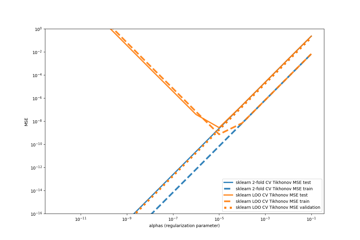
We can see that Leave-one-out CV is estimating the error wrong for low alpha values. That seems to be a numerical instability of the method. If we would have limit our alphas to 1E-5, then LOO CV would have reach similar accuracies as the 2-fold method.

Important to note that this is not an fully encompasing comparison covering sufficient enough the parameter space. We just want to note that in cases with high feature size and low effective rank the ridge solvers in skmatter can be numerical more stable and act on a comparable speed.

Cutoff and Tikhonov regularization

When using a hard threshold as regularization (using parameter cutoff), the singular values below \(\lambda\) are cut off, the size of the matrices \(\mathbf{A}_1\) and \(\mathbf{B}_1\) can then be reduced, resulting in further computation time savings. This performance advantage of cutoff over the tikhonov is visible if we to predict multiple targets and use a regularization range that cuts off a lot of singular values. For that we increase the feature size and use as regression task the prediction of a shuffled version of \(\mathbf{X}\).

X, y = make_regression(
    n_samples=1000,
    n_features=400,
    n_informative=400,
    effective_rank=5,  # decreasiing effective rank
    tail_strength=1e-9,
    random_state=SEED,
)

idx = np.arange(X.shape[1])
np.random.seed(SEED)
np.random.shuffle(idx)
y = X.copy()[:, idx]

singular_values = np.linalg.svd(X, full_matrices=False)[1]

plt.loglog(singular_values)
plt.title("Singular values of our feature matrix X")
plt.axhline(1e-8, color="gray")
plt.xlabel("index feature")
plt.ylabel("singular value")
plt.show()

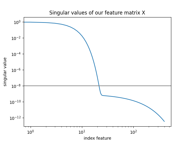
We can see that a regularization value of 1e-8 cuts off a lot of singular values. This is crucial for the computational speed up of the cutoff regularization method

# we use a denser range of regularization parameters to make
# the speed up more visible
alphas = np.geomspace(1e-8, 1e-1, 20)

cv = KFold(n_splits=2, shuffle=True, random_state=SEED)

skmatter_ridge_2foldcv_cutoff = Ridge2FoldCV(
    alphas=alphas,
    regularization_method="cutoff",
    cv=cv,
)

skmatter_ridge_2foldcv_tikhonov = Ridge2FoldCV(
    alphas=alphas,
    regularization_method="tikhonov",
    cv=cv,
)

sklearn_ridge_loocv_tikhonov = RidgeCV(
    alphas=alphas,
    cv=None,
    fit_intercept=False,  # remove the incluence of learning bias
)

print("skmatter 2-fold CV cutoff")
micro_bench(skmatter_ridge_2foldcv_cutoff)
print()
print("skmatter 2-fold CV tikhonov")
micro_bench(skmatter_ridge_2foldcv_tikhonov)
print()
print("sklearn LOO CV tikhonov")
micro_bench(sklearn_ridge_loocv_tikhonov)

skmatter 2-fold CV cutoff
  Time: 0.09898738861083985s
  Train MSE: 8.199211435485744e-23
  Test MSE: 8.313680615089296e-23

skmatter 2-fold CV tikhonov
  Time: 0.1453549385070801s
  Train MSE: 2.1125597863649234e-14
  Test MSE: 2.5492748573047085e-14

sklearn LOO CV tikhonov
  Time: 0.2146282196044922s
  Train MSE: 2.1125614894762703e-14
  Test MSE: 2.549280153596718e-14

We also want to note that these benchmarks have huge deviations per run and that more robust benchmarking methods would be adequate for this situation. However, we cannot do this here as we try to keep the computation of these examples as minimal as possible.

References

[loocv]

Rifkin “Regularized Least Squares.” https://www.mit.edu/~9.520/spring07/Classes/rlsslides.pdf