Choosing Different Regressors for PCovR

import time

from matplotlib import pyplot as plt
from sklearn.datasets import load_diabetes
from sklearn.linear_model import Ridge
from sklearn.preprocessing import StandardScaler

from skmatter.decomposition import PCovR

For this, we will use the sklearn.datasets.load_diabetes() dataset from sklearn.

mixing = 0.5

X, y = load_diabetes(return_X_y=True)

X_scaler = StandardScaler()
X_scaled = X_scaler.fit_transform(X)

y_scaler = StandardScaler()
y_scaled = y_scaler.fit_transform(y.reshape(-1, 1))

Use the default regressor in PCovR

When there is no regressor supplied, PCovR uses sklearn.linear_model.Ridge('alpha':1e-6, 'fit_intercept':False, 'tol':1e-12).

pcovr1 = PCovR(mixing=mixing, n_components=2)

t0 = time.perf_counter()
pcovr1.fit(X_scaled, y_scaled)
t1 = time.perf_counter()

print(f"Regressor is {pcovr1.regressor_} and fit took {1e3 * (t1 - t0):0.2} ms.")

Regressor is Ridge(alpha=1e-06, fit_intercept=False, tol=1e-12) and fit took 2.3 ms.

Use a fitted regressor

You can pass a fitted regressor to PCovR to rely on the predetermined regression parameters. Currently, scikit-matter supports scikit-learn classes class:LinearModel <sklearn.linear_model.LinearModel>, Ridge, and class:RidgeCV <sklearn.linear_model.RidgeCV>, with plans to support any regressor with similar architecture in the future.

regressor = Ridge(alpha=1e-6, fit_intercept=False, tol=1e-12)

t0 = time.perf_counter()
regressor.fit(X_scaled, y_scaled)
t1 = time.perf_counter()

print(f"Fit took {1e3 * (t1 - t0):0.2} ms.")

Fit took 0.61 ms.

pcovr2 = PCovR(mixing=mixing, n_components=2, regressor=regressor)

t0 = time.perf_counter()
pcovr2.fit(X_scaled, y_scaled)
t1 = time.perf_counter()

print(f"Regressor is {pcovr2.regressor_} and fit took {1e3 * (t1 - t0):0.2} ms.")

Regressor is Ridge(alpha=1e-06, fit_intercept=False, tol=1e-12) and fit took 0.99 ms.

Use a pre-predicted y

With regressor='precomputed', you can pass a regression output \(\hat{Y}\) and optional regression weights \(W\) to PCovR. If W=None, then PCovR will determine \(W\) as the least-squares solution between \(X\) and \(\hat{Y}\).

regressor = Ridge(alpha=1e-6, fit_intercept=False, tol=1e-12)

t0 = time.perf_counter()
regressor.fit(X_scaled, y_scaled)
t1 = time.perf_counter()

print(f"Fit took {1e3 * (t1 - t0):0.2} ms.")

W = regressor.coef_

Fit took 0.55 ms.

pcovr3 = PCovR(mixing=mixing, n_components=2, regressor="precomputed")

t0 = time.perf_counter()
pcovr3.fit(X_scaled, y_scaled, W=W)
t1 = time.perf_counter()

print(f"Fit took {1e3 * (t1 - t0):0.2} ms.")

Fit took 0.64 ms.

Comparing Results

Because we used the same regressor in all three models, they will yield the same result.

fig, (ax1, ax2, ax3) = plt.subplots(1, 3, figsize=(12, 4), sharex=True, sharey=True)

ax1.scatter(*pcovr1.transform(X_scaled).T, c=y)
ax2.scatter(*pcovr2.transform(X_scaled).T, c=y)
ax3.scatter(*pcovr3.transform(X_scaled).T, c=y)

ax1.set_ylabel("PCov$_2$")
ax1.set_xlabel("PCov$_1$")
ax2.set_xlabel("PCov$_1$")
ax3.set_xlabel("PCov$_1$")

ax1.set_title("Default Regressor")
ax2.set_title("Pre-fit Regressor")
ax3.set_title("Precomputed Regression Result")

fig.show()

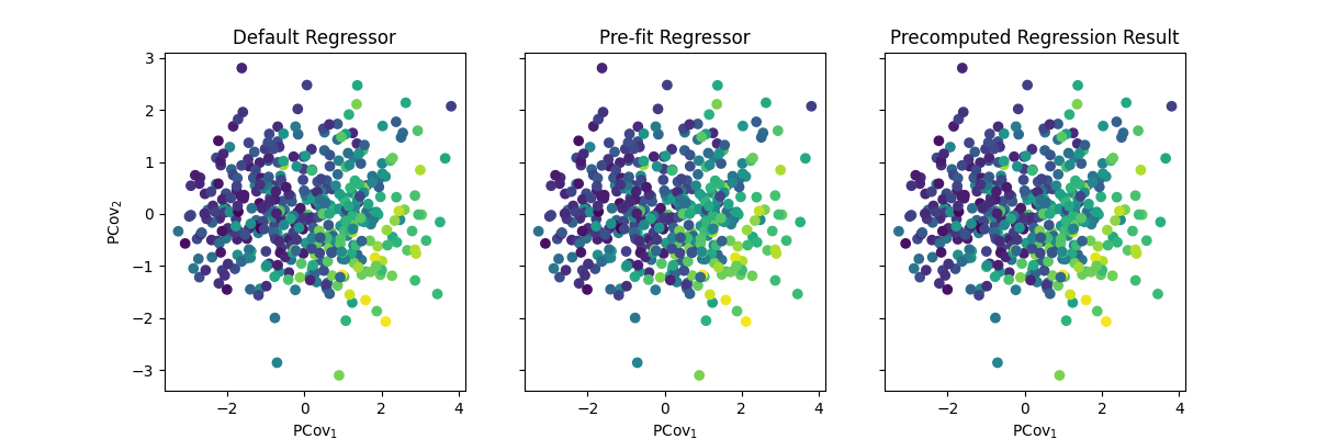
As you can imagine, these three options have different use cases – if you are working with a large dataset, you should always pre-fit to save on time!