Pointwise Local Reconstruction Error

Example for the usage of the skmatter.metrics.pointwise_local_reconstruction_error as pointwise local reconstruction error (LFRE) on the degenerate CH4 manifold. We apply the local reconstruction measure on the degenerate CH4 manifold dataset. This dataset was specifically constructed to be representable by a 4-body features (bispectrum) but not by a 3-body features (power spectrum). In other words the dataset contains environments which are different, but have the same 3-body features. For more details about the dataset please refer to Pozdnyakov 2020.

The skmatter dataset already contains the 3 and 4-body features computed with librascal so we can load it and compare it with the LFRE.

import matplotlib as mpl
import matplotlib.pyplot as plt
import numpy as np

from skmatter.datasets import load_degenerate_CH4_manifold
from skmatter.metrics import pointwise_local_reconstruction_error


mpl.rc("font", size=20)


# load features
degenerate_manifold = load_degenerate_CH4_manifold()
power_spectrum_features = degenerate_manifold.data.SOAP_power_spectrum
bispectrum_features = degenerate_manifold.data.SOAP_bispectrum

print(degenerate_manifold.DESCR)

.. _degenerate_manifold:

Degenerate CH4 manifold
#######################

The dataset contains two representations (SOAP power spectrum and bispectrum) of the two
manifolds spanned by the carbon atoms of two times 81 methane structures. The SOAP power
spectrum representation the two manifolds intersect creating a degenerate manifold/line
for which the representation remains the same. In contrast for higher body order
representations as the (SOAP) bispectrum the carbon atoms can be uniquely represented
and do not create a degenerate manifold. Following the naming convention of
[Pozdnyakov2020]_ for each representation the first 81 samples correspond to the X minus
manifold and the second 81 samples contain the X plus manifold

Function Call
-------------

.. function:: skmatter.datasets.load_degenerate_CH4_manifold

Data Set Characteristics
------------------------

:Number of Instances: Each representation 162

:Number of Features: Each  representation 12

The representations were computed with [D1]_ using the hyperparameters:

:rascal hyperparameters:

+---------------------------+------------+
| key                       |   value    |
+===========================+============+
| radial_basis:             |    "GTO"   |
+---------------------------+------------+
| interaction_cutoff:       |      4     |
+---------------------------+------------+
| max_radial:               |      2     |
+---------------------------+------------+
| max_angular:              |      2     |
+---------------------------+------------+
| gaussian_sigma_constant": |     0.5    |
+---------------------------+------------+
| gaussian_sigma_type:      |  "Constant"|
+---------------------------+------------+
| cutoff_smooth_width:      |     0.5    |
+---------------------------+------------+
| normalize:                |    False   |
+---------------------------+------------+

The SOAP bispectrum features were in addition reduced to 12 features with principal
component analysis (PCA) [D2]_.

References
----------

.. [D1] https://github.com/lab-cosmo/librascal commit 8d9ad7a
.. [D2] https://scikit-learn.org/stable/modules/generated/sklearn.decomposition.PCA.html

n_local_points = 20

print("Computing pointwise LFRE...")

Computing pointwise LFRE...

# local reconstruction error of power spectrum features using bispectrum features
power_spectrum_to_bispectrum_pointwise_lfre = pointwise_local_reconstruction_error(
    power_spectrum_features,
    bispectrum_features,
    n_local_points,
    train_idx=np.arange(0, len(power_spectrum_features), 2),
    test_idx=np.arange(0, len(power_spectrum_features)),
    estimator=None,
    n_jobs=4,
)

# local reconstruction error of bispectrum features using power spectrum features
bispectrum_to_power_spectrum_pointwise_lfre = pointwise_local_reconstruction_error(
    bispectrum_features,
    power_spectrum_features,
    n_local_points,
    train_idx=np.arange(0, len(power_spectrum_features), 2),
    test_idx=np.arange(0, len(power_spectrum_features)),
    estimator=None,
    n_jobs=4,
)

print("Computing pointwise LFRE finished.")

print(
    "LFRE(3-body, 4-body) = ",
    np.linalg.norm(power_spectrum_to_bispectrum_pointwise_lfre)
    / np.sqrt(len(power_spectrum_to_bispectrum_pointwise_lfre)),
)

print(
    "LFRE(4-body, 3-body) = ",
    np.linalg.norm(bispectrum_to_power_spectrum_pointwise_lfre)
    / np.sqrt(len(power_spectrum_to_bispectrum_pointwise_lfre)),
)

Computing pointwise LFRE finished.
LFRE(3-body, 4-body) =  0.17171573166237716
LFRE(4-body, 3-body) =  2.942859594116639e-10

fig, (ax34, ax43) = plt.subplots(
    1, 2, constrained_layout=True, figsize=(16, 7.5), sharey="row", sharex=True
)

vmax = 0.5

X, Y = np.meshgrid(np.linspace(0.7, 0.9, 9), np.linspace(-0.1, 0.1, 9))
pcm = ax34.contourf(
    X,
    Y,
    power_spectrum_to_bispectrum_pointwise_lfre[81:].reshape(9, 9).T,
    vmin=0,
    vmax=vmax,
)

ax43.contourf(
    X,
    Y,
    bispectrum_to_power_spectrum_pointwise_lfre[81:].reshape(9, 9).T,
    vmin=0,
    vmax=vmax,
)

ax34.axhline(y=0, color="red", linewidth=5)
ax43.axhline(y=0, color="red", linewidth=5)
ax34.set_ylabel(r"v/$\pi$")
ax34.set_xlabel(r"u/$\pi$")
ax43.set_xlabel(r"u/$\pi$")

ax34.set_title(r"$X^-$ LFRE(3-body, 4-body)")
ax43.set_title(r"$X^-$ LFRE(4-body, 3-body)")

cbar = fig.colorbar(pcm, ax=[ax34, ax43], label="LFRE", location="bottom")

plt.show()

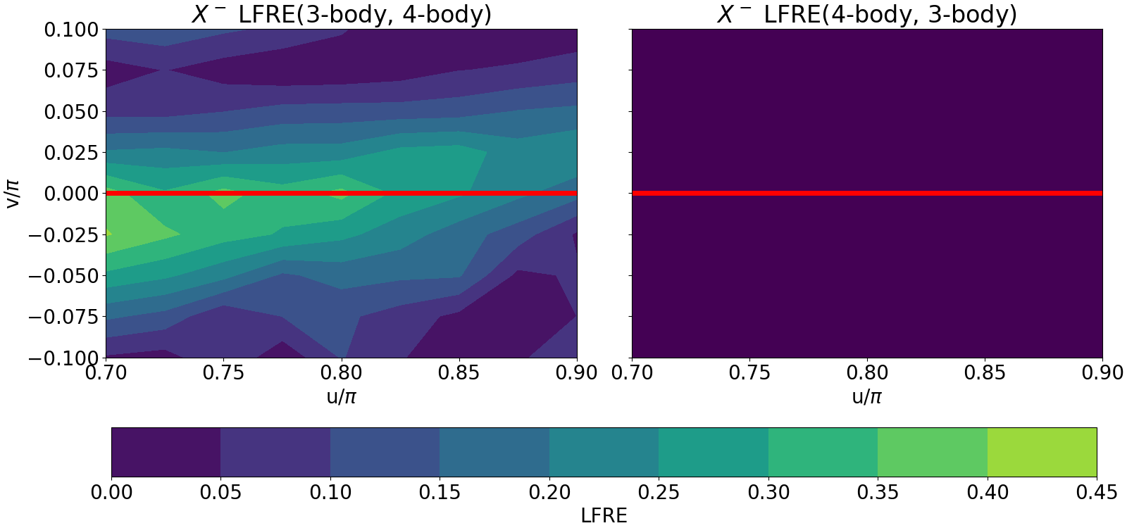
The environments span a manifold which is described by the coordinates \(v/\pi\) and \(u/\pi\) (please refer to Pozdnyakov 2020 for a concrete understanding of the manifold). The LFRE is presented for each environment in the manifold in the two contour plots. It can be seen that the reconstruction error of 4-body features using 3-body features (the left plot) is most significant along the degenerate line (the horizontal red line). This agrees with the fact that the 3-body features remain the same on the degenerate line and can therefore not reconstruct the 4-body features. On the other hand the 4-body features can perfectly reconstruct the 3-body features as seen in the right plot.