Comparing KPCovC with KPCA

import numpy as np

import matplotlib.pyplot as plt
import matplotlib as mpl
from matplotlib.colors import ListedColormap

from sklearn import datasets
from sklearn.preprocessing import StandardScaler
from sklearn.svm import LinearSVC
from sklearn.decomposition import PCA, KernelPCA
from sklearn.inspection import DecisionBoundaryDisplay
from sklearn.model_selection import train_test_split
from sklearn.linear_model import (
    LogisticRegressionCV,
    RidgeClassifierCV,
    SGDClassifier,
)

from skmatter.decomposition import PCovC, KernelPCovC

plt.rcParams["scatter.edgecolors"] = "k"
cm_bright = ListedColormap(["#d7191c", "#fdae61", "#a6d96a", "#3a7cdf"])

random_state = 0
n_components = 2

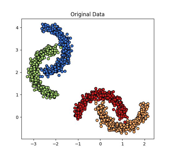
For this, we will combine two sklearn datasets from sklearn.datasets.make_moons().

X1, y1 = datasets.make_moons(n_samples=750, noise=0.10, random_state=random_state)
X2, y2 = datasets.make_moons(n_samples=750, noise=0.10, random_state=random_state)

X2, y2 = X2 + 2, y2 + 2
R = np.array(
    [
        [np.cos(np.pi / 2), -np.sin(np.pi / 2)],
        [np.sin(np.pi / 2), np.cos(np.pi / 2)],
    ]
)
# rotate second pair of moons
X2 = X2 @ R.T

X = np.vstack([X1, X2])
y = np.concatenate([y1, y2])

Original Data

fig, ax = plt.subplots(figsize=(5.5, 5))
ax.scatter(X[:, 0], X[:, 1], c=y, cmap=cm_bright)
ax.set_title("Original Data")

Text(0.5, 1.0, 'Original Data')

Scale Data

X_train, X_test, y_train, y_test = train_test_split(
    X, y, test_size=0.25, stratify=y, random_state=random_state
)

scaler = StandardScaler()
X_train_scaled = scaler.fit_transform(X_train)
X_test_scaled = scaler.transform(X_test)

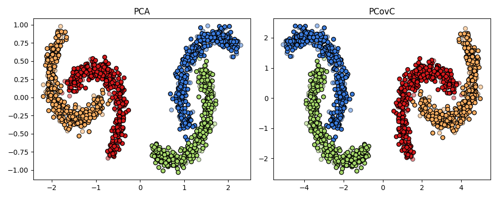
PCA and PCovC

Both PCA and PCovC fail to produce linearly separable latent space maps. We will need a kernel method to effectively separate the moon classes.

mixing = 0.10
alpha_d = 0.5
alpha_p = 0.4

models = {
    PCA(n_components=n_components): "PCA",
    PCovC(
        n_components=n_components,
        random_state=random_state,
        mixing=mixing,
        classifier=LinearSVC(),
    ): "PCovC",
}

fig, axs = plt.subplots(1, 2, figsize=(10, 4))

for ax, model in zip(axs, models):
    t_train = model.fit_transform(X_train_scaled, y_train)
    t_test = model.transform(X_test_scaled)

    ax.scatter(t_test[:, 0], t_test[:, 1], alpha=alpha_d, cmap=cm_bright, c=y_test)
    ax.scatter(t_train[:, 0], t_train[:, 1], cmap=cm_bright, c=y_train)

    ax.set_title(models[model])
    plt.tight_layout()

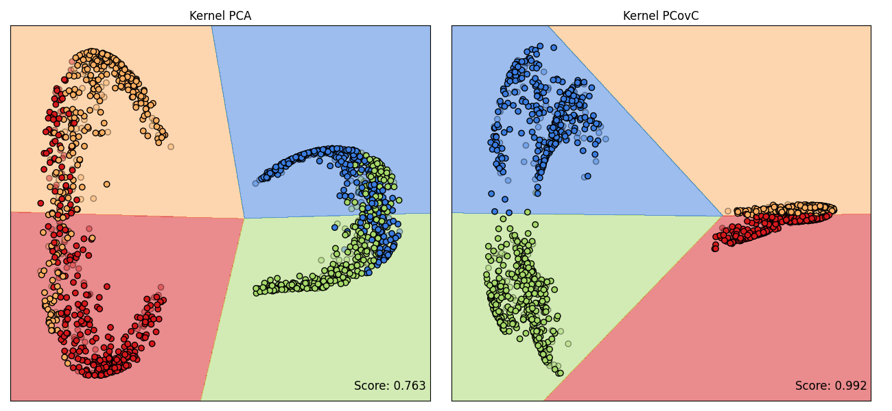
Kernel PCA and Kernel PCovC

A comparison of the latent spaces produced by KPCA and KPCovC is shown. A logistic regression classifier is trained on the KPCA latent space (this is also the default classifier used in KPCovC), and we see the comparison of the respective decision boundaries and test data accuracy scores.

fig, axs = plt.subplots(1, 2, figsize=(13, 6))

center = True
resolution = 1000

kernel_params = {"kernel": "rbf", "gamma": 2}

models = {
    KernelPCA(n_components=n_components, **kernel_params): {
        "title": "Kernel PCA",
        "eps": 0.1,
    },
    KernelPCovC(
        n_components=n_components,
        random_state=random_state,
        mixing=mixing,
        center=center,
        **kernel_params,
    ): {"title": "Kernel PCovC", "eps": 2},
}

for ax, model in zip(axs, models):
    t_train = model.fit_transform(X_train_scaled, y_train)
    t_test = model.transform(X_test_scaled)

    if isinstance(model, KernelPCA):
        t_classifier = LinearSVC(random_state=random_state).fit(t_train, y_train)
        score = t_classifier.score(t_test, y_test)
    else:
        t_classifier = model.classifier_
        score = model.score(X_test_scaled, y_test)

    DecisionBoundaryDisplay.from_estimator(
        estimator=t_classifier,
        X=t_test,
        ax=ax,
        response_method="predict",
        cmap=cm_bright,
        alpha=alpha_d,
        eps=models[model]["eps"],
        grid_resolution=resolution,
    )
    ax.scatter(t_test[:, 0], t_test[:, 1], alpha=alpha_p, cmap=cm_bright, c=y_test)
    ax.scatter(t_train[:, 0], t_train[:, 1], cmap=cm_bright, c=y_train)
    ax.set_title(models[model]["title"])

    ax.text(
        0.82,
        0.03,
        f"Score: {round(score, 3)}",
        fontsize=mpl.rcParams["axes.titlesize"],
        transform=ax.transAxes,
    )
    ax.set_xticks([])
    ax.set_yticks([])

fig.subplots_adjust(wspace=0.04)
plt.tight_layout()

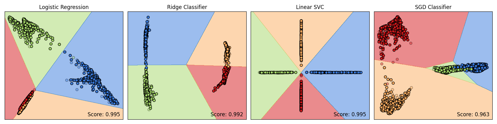
Effect of KPCovC Classifier on KPCovC Maps and Decision Boundaries

Based on the evidence \(\mathbf{Z}\) generated by the underlying classifier fit on a computed kernel \(\mathbf{K}\) and \(\mathbf{Y}\), Kernel PCovC will produce varying latent space maps. Hence, the decision boundaries produced by the linear classifier fit between \(\mathbf{T}\) and \(\mathbf{Y}\) to make predictions will also vary.

names = ["Logistic Regression", "Ridge Classifier", "Linear SVC", "SGD Classifier"]

models = {
    LogisticRegressionCV(random_state=random_state): {
        "kernel_params": {"kernel": "rbf", "gamma": 12},
        "title": "Logistic Regression",
    },
    RidgeClassifierCV(): {
        "kernel_params": {"kernel": "rbf", "gamma": 1},
        "title": "Ridge Classifier",
        "eps": 0.40,
    },
    LinearSVC(random_state=random_state): {
        "kernel_params": {"kernel": "rbf", "gamma": 15},
        "title": "Support Vector Classification",
    },
    SGDClassifier(random_state=random_state): {
        "kernel_params": {"kernel": "rbf", "gamma": 15},
        "title": "SGD Classifier",
        "eps": 10,
    },
}

fig, axs = plt.subplots(1, len(models), figsize=(4 * len(models), 4))

for ax, name, model in zip(axs.flat, names, models):
    kpcovc = KernelPCovC(
        n_components=n_components,
        random_state=random_state,
        mixing=mixing,
        classifier=model,
        center=center,
        **models[model]["kernel_params"],
    )
    t_kpcovc_train = kpcovc.fit_transform(X_train_scaled, y_train)
    t_kpcovc_test = kpcovc.transform(X_test_scaled)
    kpcovc_score = kpcovc.score(X_test_scaled, y_test)

    DecisionBoundaryDisplay.from_estimator(
        estimator=kpcovc.classifier_,
        X=t_kpcovc_test,
        ax=ax,
        response_method="predict",
        cmap=cm_bright,
        alpha=alpha_d,
        eps=models[model].get("eps", 1),
        grid_resolution=resolution,
    )

    ax.scatter(
        t_kpcovc_test[:, 0],
        t_kpcovc_test[:, 1],
        cmap=cm_bright,
        alpha=alpha_p,
        c=y_test,
    )
    ax.scatter(t_kpcovc_train[:, 0], t_kpcovc_train[:, 1], cmap=cm_bright, c=y_train)
    ax.text(
        0.70,
        0.03,
        f"Score: {round(kpcovc_score, 3)}",
        fontsize=mpl.rcParams["axes.titlesize"],
        transform=ax.transAxes,
    )

    ax.set_title(name)
    ax.set_xticks([])
    ax.set_yticks([])
    fig.subplots_adjust(wspace=0.04)

    plt.tight_layout()