PCovC Hyperparameter Tuning

import matplotlib.pyplot as plt
from matplotlib.colors import LinearSegmentedColormap
from sklearn.datasets import load_iris
from sklearn.decomposition import PCA
from sklearn.inspection import DecisionBoundaryDisplay
from sklearn.linear_model import LogisticRegressionCV, Perceptron, RidgeClassifierCV
from sklearn.preprocessing import StandardScaler
from sklearn.svm import LinearSVC

from skmatter.decomposition import PCovC


plt.rcParams["image.cmap"] = "tab10"
plt.rcParams["scatter.edgecolors"] = "k"

random_state = 10
n_components = 2

For this, we will use the sklearn.datasets.load_iris() dataset from sklearn.

X, y = load_iris(return_X_y=True)

scaler = StandardScaler()
X_scaled = scaler.fit_transform(X)

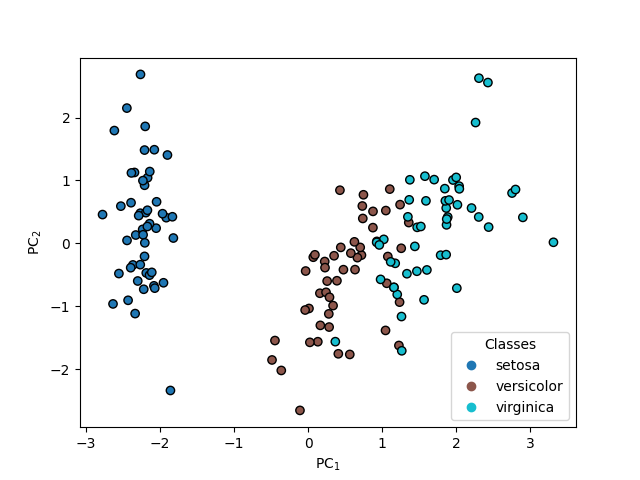
PCA

pca = PCA(n_components=n_components)

pca.fit(X_scaled, y)
T_pca = pca.transform(X_scaled)

fig, axis = plt.subplots()
scatter = axis.scatter(T_pca[:, 0], T_pca[:, 1], c=y)
axis.set(xlabel="PC$_1$", ylabel="PC$_2$")
axis.legend(
    scatter.legend_elements()[0],
    load_iris().target_names,
    loc="lower right",
    title="Classes",
)

<matplotlib.legend.Legend object at 0x7ee561fb0e10>

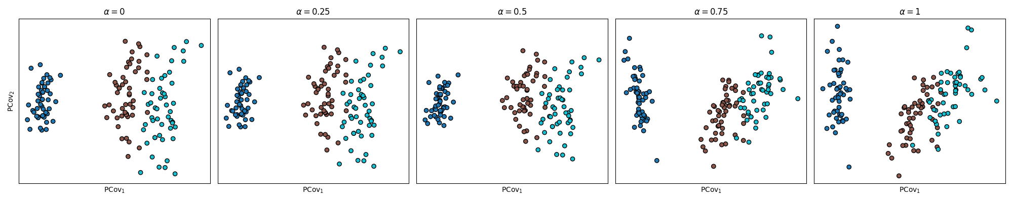
Effect of Mixing Parameter \(\alpha\) on PCovC Map

Below, we see how different \(\alpha\) values for our PCovC model result in varying class distinctions between setosa, versicolor, and virginica on the PCovC map.

n_mixing = 5
mixing_params = [0, 0.25, 0.50, 0.75, 1]

fig, axs = plt.subplots(1, n_mixing, figsize=(4 * n_mixing, 4), sharey="row")

for ax, mixing in zip(axs, mixing_params):
    pcovc = PCovC(
        mixing=mixing,
        n_components=n_components,
        random_state=random_state,
        classifier=LogisticRegressionCV(),
    )

    pcovc.fit(X_scaled, y)
    T = pcovc.transform(X_scaled)

    ax.set_xticks([])
    ax.set_yticks([])

    ax.set_title(r"$\alpha=$" + str(mixing))
    ax.set_xlabel("PCov$_1$")
    ax.scatter(T[:, 0], T[:, 1], c=y)

axs[0].set_ylabel("PCov$_2$")

fig.subplots_adjust(wspace=0)
plt.tight_layout()

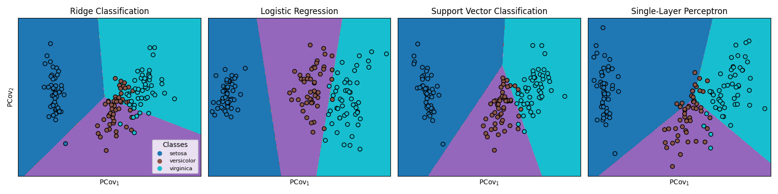
Effect of PCovC Classifier on PCovC Maps and Decision Boundaries

Here, we see how a PCovC model (\(\alpha\) = 0.5) fitted with different classifiers produces varying PCovC maps. In addition, we see the varying decision boundaries produced by the respective PCovC classifiers.

mixing = 0.5
fig, axs = plt.subplots(1, 4, figsize=(16, 4))

models = {
    RidgeClassifierCV(): "Ridge Classification",
    LogisticRegressionCV(random_state=random_state): "Logistic Regression",
    LinearSVC(random_state=random_state): "Support Vector Classification",
    Perceptron(random_state=random_state): "Single-Layer Perceptron",
}

for ax, model in zip(axs, models):
    pcovc = PCovC(
        mixing=mixing,
        n_components=n_components,
        random_state=random_state,
        classifier=model,
    )

    pcovc.fit(X_scaled, y)
    T = pcovc.transform(X_scaled)

    ax.set_title(models[model])

    DecisionBoundaryDisplay.from_estimator(
        estimator=pcovc.classifier_,
        X=T,
        ax=ax,
        response_method="predict",
        grid_resolution=1000,
    )

    scatter = ax.scatter(T[:, 0], T[:, 1], c=y)

    ax.set_xlabel("PCov$_1$")
    ax.set_xticks([])
    ax.set_yticks([])

axs[0].set_ylabel("PCov$_2$")
axs[0].legend(
    scatter.legend_elements()[0],
    load_iris().target_names,
    loc="lower right",
    title="Classes",
    fontsize=8,
)

fig.subplots_adjust(wspace=0.04)
plt.tight_layout()
plt.show()