Pointwise GFRE applied on RKHS features

Example for the usage of the skmatter.metrics.pointwise_global_reconstruction_error as the pointwise global feature reconstruction error (pointwise GFRE). We apply the pointwise global feature reconstruction error on the degenerate CH4 manifold dataset containing 3 and 4-body features computed with librascal. We will show that using reproducing kernel Hilbert space (RKHS) features can improve the quality of the reconstruction with the downside of being less general.

import matplotlib as mpl
import matplotlib.pyplot as plt
import numpy as np
from sklearn.model_selection import train_test_split
from sklearn.preprocessing._data import KernelCenterer

from skmatter.datasets import load_degenerate_CH4_manifold
from skmatter.metrics import (
    global_reconstruction_error,
    pointwise_global_reconstruction_error,
)
from skmatter.preprocessing import StandardFlexibleScaler


mpl.rc("font", size=20)

# load features
degenerate_manifold = load_degenerate_CH4_manifold()
power_spectrum_features = degenerate_manifold.data.SOAP_power_spectrum
bispectrum_features = degenerate_manifold.data.SOAP_bispectrum

We compare 3-body features with their mapping to the reproducing kernel Hilbert space (RKHS) projected to the sample space using the nonlinear radial basis function (RBF) kernel

\[k^{\textrm{RBF}}(\mathbf{x},\mathbf{x}') = \exp(-\gamma \|\mathbf{x}-\mathbf{x}'\|^2),\quad \gamma\in\mathbb{R}_+\]

The projected RKHS features are computed using the eigendecomposition of the positive-definite kernel matrix \(K\)

\[K = ADA^T = AD^{\frac12}(AD^{\frac12})^T = \Phi\Phi^T\]

def compute_standardized_rbf_rkhs_features(features, gamma):
    """Compute the  standardized RDF RKHS features."""
    # standardize features
    features = StandardFlexibleScaler().fit_transform(features)

    # compute \|x - x\|^2
    squared_distance = (
        np.sum(features**2, axis=1)[:, np.newaxis]
        + np.sum(features**2, axis=1)[np.newaxis, :]
        - 2 * features.dot(features.T)
    )
    # computer rbf kernel
    kernel = np.exp(-gamma * squared_distance)

    # center kernel
    kernel = KernelCenterer().fit_transform(kernel)

    # compute D and A
    D, A = np.linalg.eigh(kernel)

    # retain features associated with an eigenvalue above 1e-9 for denoising
    select_idx = np.where(D > 1e-9)[0]

    # compute rkhs features
    rbf_rkhs_features = A[:, select_idx] @ np.diag(np.sqrt(D[select_idx]))

    # standardize rkhs features,
    # this step could be omitted since it is done by the reconstruction measure by
    # default
    standardized_rbf_rkhs_features = StandardFlexibleScaler().fit_transform(
        rbf_rkhs_features
    )
    return standardized_rbf_rkhs_features


gamma = 1
rbf_power_spectrum_features = compute_standardized_rbf_rkhs_features(
    power_spectrum_features, gamma=gamma
)

# some split into train and test idx
idx = np.arange(len(power_spectrum_features))

train_idx, test_idx = train_test_split(idx, random_state=42)

print("Computing pointwise GFRE...")

# pointwise global reconstruction error of bispectrum features using power spectrum
# features
power_spectrum_to_bispectrum_pointwise_gfre = pointwise_global_reconstruction_error(
    power_spectrum_features, bispectrum_features, train_idx=train_idx, test_idx=test_idx
)

# pointwise global reconstruction error of bispectrum features using power spectrum
# features mapped to the RKHS
power_spectrum_rbf_to_bispectrum_pointwise_gfre = pointwise_global_reconstruction_error(
    rbf_power_spectrum_features,
    bispectrum_features,
    train_idx=train_idx,
    test_idx=test_idx,
)

print("Computing pointwise GFRE finished.")

print("Computing GFRE...")

# global reconstruction error of bispectrum features using power spectrum features
power_spectrum_to_bispectrum_gfre = global_reconstruction_error(
    power_spectrum_features, bispectrum_features, train_idx=train_idx, test_idx=test_idx
)

# global reconstruction error of bispectrum features using power spectrum features
# mapped to the RKHS
power_spectrum_rbf_to_bispectrum_gfre = global_reconstruction_error(
    rbf_power_spectrum_features,
    bispectrum_features,
    train_idx=train_idx,
    test_idx=test_idx,
)

print("Computing GFRE finished.")

Computing pointwise GFRE...
Computing pointwise GFRE finished.
Computing GFRE...
Computing GFRE finished.

fig, axes = plt.subplots(1, 1, figsize=(12, 7))

bins = np.linspace(0, 0.5, 10)
axes.hist(
    power_spectrum_to_bispectrum_pointwise_gfre,
    bins,
    alpha=0.5,
    label="pointwise GFRE(3-body, 4-body)",
)
axes.hist(
    power_spectrum_rbf_to_bispectrum_pointwise_gfre,
    bins,
    color="r",
    alpha=0.5,
    label="pointwise GFRE(3-body RBF, 4-body)",
)
axes.axvline(
    power_spectrum_to_bispectrum_gfre,
    color="darkblue",
    label="GFRE(3-body, 4-body)",
    linewidth=4,
)
axes.axvline(
    power_spectrum_rbf_to_bispectrum_gfre,
    color="darkred",
    label="GFRE(3-body RBF RKHS, 4-body)",
    linewidth=4,
)
axes.set_title(f"3-body vs 4-body RBF gamma={gamma} comparison")
axes.set_xlabel("pointwise GFRE")
axes.set_ylabel("number of samples")
axes.legend(fontsize=13)
plt.show()

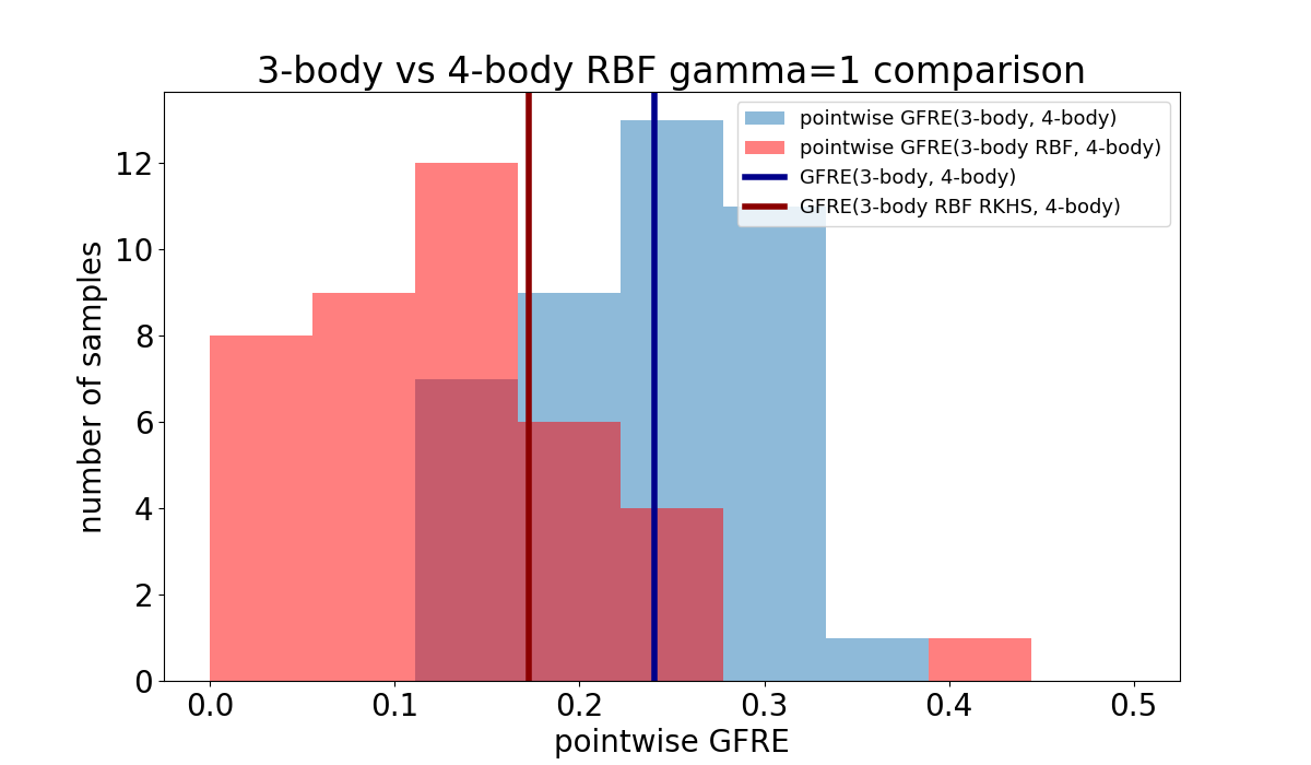
print("GFRE(3-body, 4-body) =", power_spectrum_to_bispectrum_gfre)
print("GFRE(3-body RBF RKHS, 4-body) = ", power_spectrum_rbf_to_bispectrum_gfre)

GFRE(3-body, 4-body) = 0.24067762664477704
GFRE(3-body RBF RKHS, 4-body) =  0.17263420660595977

It can be seen that RBF RKHS features improve the linear reconstruction of the 4-body features (~0.22 in contrast to ~0.19) while also spreading the error for individual samples across a wider span of [0, 0.45] in contrast to [0.17, 0.32]. This indicates that the reconstruction using the RBF RKHS is less generally applicable but instead specific to this dataset