Note
Go to the end to download the full example code.
Generalized Convex Hull construction for the polymorphs of ROY#
This notebook analyzes the structures of 264 polymorphs of ROY, from Beran et Al, Chemical Science (2022), comparing the conventional density-energy convex hull with a Generalized Convex Hull (GCH) analysis (see Anelli et al., Phys. Rev. Materials (2018)).
import matplotlib.tri as mtri
import numpy as np
from matplotlib import pyplot as plt
from sklearn.decomposition import PCA

from skmatter.datasets import load_roy_dataset
from skmatter.sample_selection import DirectionalConvexHull
Loads the structures (that also contain properties in the info
field)
Energy-density hull#
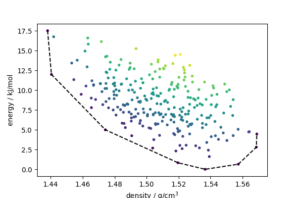
The Directional Convex Hull routines can be used to compute a conventional density-energy hull
dch_builder = DirectionalConvexHull(low_dim_idx=[0])
dch_builder.fit(density.reshape(-1, 1), energy)
We can get the indices of the selection, and compute the distance from the hull
sel = dch_builder.selected_idx_
dch_dist = dch_builder.score_samples(density.reshape(-1, 1), energy)
Structures on the hull are stable with respect to synthesis at constant molar volume. Any other structure would lower the energy by decomposing into a mixture of the two nearest structures along the hull. Given that the lattice energy is an imperfect proxy for the free energy, and that synthesis can be performed in other ways than by fixing the density, structures that are not exactly on the hull might also be stable. One can compute a “hull energy” as an indication of how close these structures are to being stable .
fig, ax = plt.subplots(1, 1, figsize=(6, 4))
ax.scatter(density, energy, c=dch_dist, marker=".")
ssel = sel[np.argsort(density[sel])]
ax.plot(density[ssel], energy[ssel], "k--")
ax.set_xlabel("density / g/cm$^3$")
ax.set_ylabel("energy / kJ/mol")

print(
    f"Mean hull energy for 'known' stable structures {dch_dist[iknown].mean()} kJ/mol"
)
print(f"Mean hull energy for 'other' structures {dch_dist[iothers].mean()} kJ/mol")
Mean hull energy for 'known' stable structures 1.816657381014075 kJ/mol
Mean hull energy for 'other' structures 6.312730486304906 kJ/mol
You can also visualize the hull with chemiscope.
This runs only in a notebook, and
requires having the chemiscope package installed.
"""
import chemiscope
chemiscope.show(
    structures,
    dict(
        energy=energy, density=density,
        hull_energy=dch_dist, structure_type=structype
    ),
    settings={
        "map": {
               "x": {"property": "density"},
               "y": {"property": "energy"},
               "color": {"property": "hull_energy"},
               "symbol": "structure_type",
               "size": {"factor": 35},
        },
        "structure": [{"unitCell": True, "supercell": {"0": 2, "1": 2, "2": 2}}],
    },
)
"""
'\nimport chemiscope\nchemiscope.show(\n structures,\n dict(\n energy=energy, density=density,\n hull_energy=dch_dist, structure_type=structype\n ),\n settings={\n "map": {\n "x": {"property": "density"},\n "y": {"property": "energy"},\n "color": {"property": "hull_energy"},\n "symbol": "structure_type",\n "size": {"factor": 35},\n },\n "structure": [{"unitCell": True, "supercell": {"0": 2, "1": 2, "2": 2}}],\n },\n)\n'
Generalized Convex Hull#
A GCH is a similar construction, in which generic structural descriptors are used in lieu of composition, density or other thermodynamic constraints. The idea is that configurations that are found close to the GCH are locally stable with respect to structurally-similar configurations. In other terms, one can hope to find a thermodynamic constraint (i.e. synthesis conditions) that act differently on these structures in comparison with the others, and may potentially stabilize them.
A first step is to computes suitable ML descriptors. Here we have used
rascaline to evaluate average SOAP features for the structures. We
will load pre-computed features to reduce the dependencies of these
examples on external packages, but you can use this as a stub to apply
this analysis to other chemical systems
"""
from rascaline import SoapPowerSpectrum
from equistore import mean_over_samples
hypers = {
    "cutoff": 4,
    "max_radial": 6,
    "max_angular": 4,
    "atomic_gaussian_width": 0.7,
    "cutoff_function": {"ShiftedCosine": {"width": 0.5}},
    "radial_basis": {"Gto": {"accuracy": 1e-6}},
    "center_atom_weight": 1.0
}
calculator = SoapPowerSpectrum(**hypers)
rho2i = calculator.compute(structures)
rho2i=rho2i.keys_to_samples(['species_center']).keys_to_properties(
                   ['species_neighbor_1', 'species_neighbor_2'])
rho2i_structure = mean_over_samples(rho2i,
                        sample_names=["center", "species_center"])
np.savez("roy_features.npz", feats=rho2i_structure.block(0).values)
"""


features = roy_data["features"]
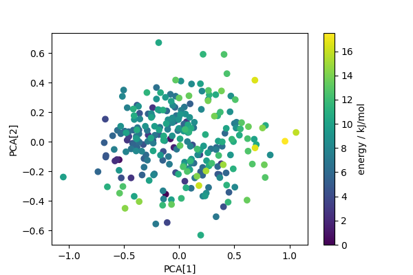
Computes PCA projection to generate low-dimensional descriptors that reflect structural diversity. Any other dimensionality reduction scheme could be used in a similar fashion.
pca = PCA(n_components=4)
pca_features = pca.fit_transform(features)

fig, ax = plt.subplots(1, 1, figsize=(6, 4))
scatter = ax.scatter(pca_features[:, 0], pca_features[:, 1], c=energy)
ax.set_xlabel("PCA[1]")
ax.set_ylabel("PCA[2]")
cbar = fig.colorbar(scatter, ax=ax)
cbar.set_label("energy / kJ/mol")
Builds a convex hull on the first two PCA features
dch_builder = DirectionalConvexHull(low_dim_idx=[0, 1])
dch_builder.fit(pca_features, energy)
sel = dch_builder.selected_idx_
dch_dist = dch_builder.score_samples(pca_features, energy)
Generates a 3D Plot
triang = mtri.Triangulation(pca_features[sel, 0], pca_features[sel, 1])
fig = plt.figure(figsize=(7, 5), tight_layout=True)
ax = fig.add_subplot(projection="3d")
ax.plot_trisurf(triang, energy[sel], color="gray")
ax.scatter(pca_features[:, 0], pca_features[:, 1], energy, c=dch_dist)
ax.set_xlabel("PCA[1]")
ax.set_ylabel("PCA[2]")
ax.set_zlabel("energy / kJ/mol\n \n", labelpad=11)
ax.view_init(25, 110)
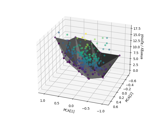
The GCH construction improves the separation between the hull energies of “known” and hypothetical polymorphs (compare with the density-energy values above)
Mean hull energy for 'known' stable structures 0.8539156846959327 kJ/mol
Mean hull energy for 'other' structures 5.19873860454363 kJ/mol
Visualize in chemiscope. This runs only in a notebook, and
requires having the chemiscope package installed.
"""
import chemiscope
for i, f in enumerate(structures):
    for j in range(len(pca_features[i])):
        f.info["pca_" + str(j + 1)] = pca_features[i, j]
structure_properties = chemiscope.extract_properties(structures)
structure_properties.update({"per_atom_energy": energy, "hull_energy": dch_dist})
chemiscope.show(
    frames=structures,
    properties=structure_properties,
    settings={
        "map": {
            "x": {"property": "pca_1"},
            "y": {"property": "pca_2"},
            "z": {"property": "energy"},
            "symbol": "type",
            "symbol": "type",
            "color": {"property": "hull_energy"},
            "size": {"factor": 35, "mode": "linear",
                     "property": "", "reverse": True},
        },
        "structure": [
            {
               "bonds": True,
               "unitCell": True,
               "keepOrientation": True,
            }
        ],
    },
)
"""
'\nimport chemiscope\nfor i, f in enumerate(structures):\n for j in range(len(pca_features[i])):\n f.info["pca_" + str(j + 1)] = pca_features[i, j]\nstructure_properties = chemiscope.extract_properties(structures)\nstructure_properties.update({"per_atom_energy": energy, "hull_energy": dch_dist})\nchemiscope.show(\n frames=structures,\n properties=structure_properties,\n settings={\n "map": {\n "x": {"property": "pca_1"},\n "y": {"property": "pca_2"},\n "z": {"property": "energy"},\n "symbol": "type",\n "symbol": "type",\n "color": {"property": "hull_energy"},\n "size": {"factor": 35, "mode": "linear",\n "property": "", "reverse": True},\n },\n "structure": [\n {\n "bonds": True,\n "unitCell": True,\n "keepOrientation": True,\n }\n ],\n },\n)\n'