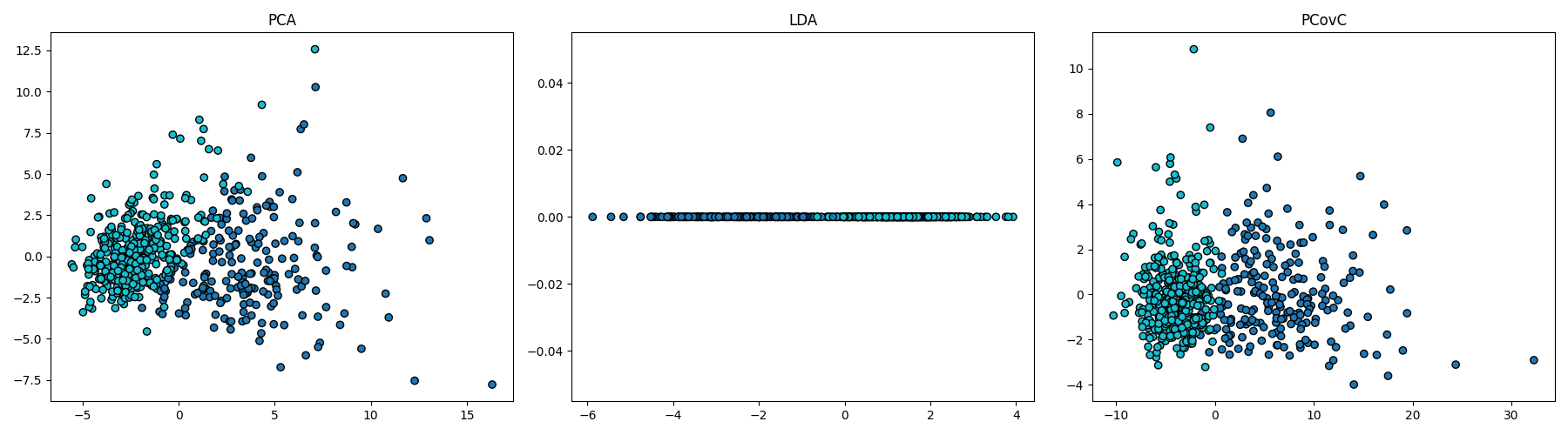
Comparing PCovC with PCA and LDA

import matplotlib.pyplot as plt
import numpy as np
from sklearn.datasets import load_breast_cancer
from sklearn.decomposition import PCA
from sklearn.discriminant_analysis import LinearDiscriminantAnalysis
from sklearn.linear_model import LogisticRegressionCV
from sklearn.preprocessing import StandardScaler

from skmatter.decomposition import PCovC


plt.rcParams["image.cmap"] = "tab10"
plt.rcParams["scatter.edgecolors"] = "k"

random_state = 0

For this, we will use the sklearn.datasets.load_breast_cancer() dataset from sklearn.

X, y = load_breast_cancer(return_X_y=True)

scaler = StandardScaler()
X_scaled = scaler.fit_transform(X)

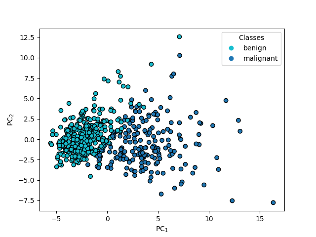
PCA

pca = PCA(n_components=2)

pca.fit(X_scaled, y)
T_pca = pca.transform(X_scaled)

fig, ax = plt.subplots()
scatter = ax.scatter(T_pca[:, 0], T_pca[:, 1], c=y)
ax.set(xlabel="PC$_1$", ylabel="PC$_2$")
ax.legend(
    scatter.legend_elements()[0][::-1],
    load_breast_cancer().target_names[::-1],
    loc="upper right",
    title="Classes",
)

<matplotlib.legend.Legend object at 0x7ee561f79810>

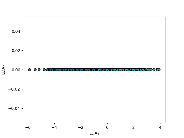
LDA

lda = LinearDiscriminantAnalysis(n_components=1)
lda.fit(X_scaled, y)

T_lda = lda.transform(X_scaled)

fig, ax = plt.subplots()
ax.scatter(T_lda[:], np.zeros(len(T_lda[:])), c=y)
ax.set(xlabel="LDA$_1$", ylabel="LDA$_2$")

[Text(0.5, 23.52222222222222, 'LDA$_1$'), Text(22.472222222222214, 0.5, 'LDA$_2$')]

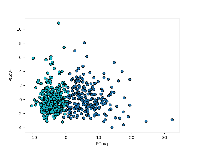
PCovC

Below, we see the map produced by a PCovC model with \(\alpha\) = 0.5 and a logistic regression classifier.

mixing = 0.5

pcovc = PCovC(
    mixing=mixing,
    n_components=2,
    random_state=random_state,
    classifier=LogisticRegressionCV(),
)
pcovc.fit(X_scaled, y)

T_pcovc = pcovc.transform(X_scaled)

fig, ax = plt.subplots()
ax.scatter(T_pcovc[:, 0], T_pcovc[:, 1], c=y)
ax.set(xlabel="PCov$_1$", ylabel="PCov$_2$")

[Text(0.5, 23.52222222222222, 'PCov$_1$'), Text(44.347222222222214, 0.5, 'PCov$_2$')]

A side-by-side comparison of the three maps (PCA, LDA, and PCovC):

fig, axs = plt.subplots(1, 3, figsize=(18, 5))
axs[0].scatter(T_pca[:, 0], T_pca[:, 1], c=y)
axs[0].set_title("PCA")
axs[1].scatter(T_lda, np.zeros(len(T_lda)), c=y)
axs[1].set_title("LDA")
axs[2].scatter(T_pcovc[:, 0], T_pcovc[:, 1], c=y)
axs[2].set_title("PCovC")

plt.tight_layout()
plt.show()