Regression with orthogonal projector/matrices

In this example, we explain how when using skmatter.linear_model.OrthogonalRegression the option use_orthogonal_projector can result in non-analytic behavior. In skmatter.linear_model.OrthogonalRegression, we solve the linear regression problem assuming an orthogonal weighting matrix \(\Omega\) to project from the feature space \(X\) to the target space \(y\).

\[\min_\Omega ||y - X\Omega\||_F\]

This assumes that \(X\) and \(y\) contain the same number of features. If use_orthogonal_projector=False, the smaller of \(X\) and \(y\) is padded with null features, i.e. columns of zeros. However, when use_orthogonal_projector=True, we begin with the weights \(W\) determined by the linear regression problem

\[\min_W ||y - XW\||F \,,\]

and solve the orthogonal Procrustes problem for

\[\min\Omega' ||yV - XU\Omega'\||_F\quad \Omega'^T\Omega'=I \,,\]

where the SVD of \(W = USV^T\). The final orthogonal projector is then \(\Omega = U\Omega' V^T\). In this notebook, we demonstrate a problem that may arise with this solution, as changing the number of features can result in non-analytic behavior of the reconstruction matrix and therefore also in the predictions.

import matplotlib as mpl
import matplotlib.pyplot as plt
import numpy as np
from mpl_toolkits.axes_grid1 import make_axes_locatable

from skmatter.linear_model import OrthogonalRegression


mpl.rc("font", size=16)

Below are coordinates of a 3-dimensional cube. We treat the points of the cube as samples and the 3 dimensions as features x, y, and z.

cube = np.array(
    [
        # x  y  z
        [0, 0, 0],
        [1, 0, 0],
        [0, 1, 0],
        [1, 1, 0],
        [0, 0, 1],
        [0, 1, 1],
        [1, 0, 1],
        [1, 1, 1],
    ]
)

The x y coordinates of the cube are obtained as follows:

xy_plane_projected_cube = cube[:, [0, 1]]

A square prism, with scaling applied on the z axis, can be defined as such:

def z_scaled_square_prism(z_scaling):
    """Scaling for a prism."""
    return np.array(
        [
            [0, 0, 0],
            [1, 0, 0],
            [0, 1, 0],
            [1, 1, 0],
            [0, 0, z_scaling],
            [0, 1, z_scaling],
            [1, 0, z_scaling],
            [1, 1, z_scaling],
        ]
    )

In terms of information retrievable by regression analysis xy_plane_projected_cube is equivalent to z_scaled_square_prism with z_scaling = 0, since adding features containing only zero values to your dataset should not change the prediction quality of the regression analysis.

We now compute the orthogonal regression error fitting on the square prism to predict the cube. In the case of a zero z-scaling, the error is computed once with a third dimension and once without it (using xy_plane_projected_cube). The regression is done with skmatter.linear_model.OrthogonalRegression with use_orthogonal_projector set to True.

z_scalings = np.linspace(0, 1, 11)

regression_errors_for_z_scaled_square_prism_using_orthogonal_projector = []
orth_reg_pred_cube = len(z_scalings) * [0]
orth_reg_using_orthogonal_projector = OrthogonalRegression(
    use_orthogonal_projector=True
)
for i, z in enumerate(z_scalings):
    orth_reg_using_orthogonal_projector.fit(cube, z_scaled_square_prism(z))
    orth_reg_pred_cube[i] = orth_reg_using_orthogonal_projector.predict(cube)
    regression_error = np.linalg.norm(z_scaled_square_prism(z) - orth_reg_pred_cube[i])
    regression_errors_for_z_scaled_square_prism_using_orthogonal_projector.append(
        regression_error
    )


orth_reg_using_orthogonal_projector.fit(cube, xy_plane_projected_cube)
orth_reg_use_projector_xy_plane_pred_cube = orth_reg_using_orthogonal_projector.predict(
    cube
)
regression_error_for_xy_plane_projected_cube_using_orthogonal_projector = (
    np.linalg.norm(xy_plane_projected_cube - orth_reg_use_projector_xy_plane_pred_cube)
)

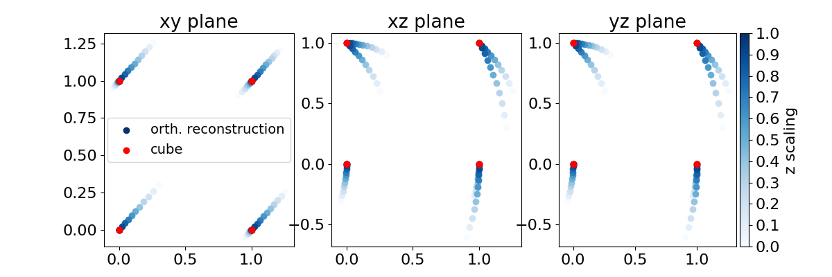
In the next cell we plot a visualization of the reconstruction of the square prism for different z scalings. We plot the projections of the xy, xz and yz planes.

fig, (ax_xy, ax_xz, ax_yz) = plt.subplots(1, 3, figsize=(12, 4))
cmap = mpl.cm.Blues
colors = cmap(np.linspace(0, 1, 11))
for i in range(len(orth_reg_pred_cube) - 1):
    ax_xy.scatter(
        orth_reg_pred_cube[i][:, 0], orth_reg_pred_cube[i][:, 1], color=colors[i]
    )
    ax_xz.scatter(
        orth_reg_pred_cube[i][:, 0], orth_reg_pred_cube[i][:, 2], color=colors[i]
    )
    ax_yz.scatter(
        orth_reg_pred_cube[i][:, 1], orth_reg_pred_cube[i][:, 2], color=colors[i]
    )

i = len(orth_reg_pred_cube) - 1
ax_xy.scatter(
    orth_reg_pred_cube[i][:, 0],
    orth_reg_pred_cube[i][:, 1],
    color=colors[i],
    label="orth. reconstruction",
)
ax_xz.scatter(orth_reg_pred_cube[i][:, 0], orth_reg_pred_cube[i][:, 2], color=colors[i])
ax_yz.scatter(orth_reg_pred_cube[i][:, 1], orth_reg_pred_cube[i][:, 2], color=colors[i])

ax_xy.scatter(cube[:, 0], cube[:, 1], c="r", label="cube")
ax_xz.scatter(cube[:, 0], cube[:, 2], c="r")
ax_yz.scatter(cube[:, 1], cube[:, 2], c="r")

ax_xy.legend(fontsize=14, loc="center")

divider = make_axes_locatable(plt.gca())
ax_cb = divider.new_horizontal(size="5%", pad=0.05)
cb1 = mpl.colorbar.ColorbarBase(
    ax_cb, cmap=cmap, orientation="vertical", ticks=z_scalings
)

plt.gcf().add_axes(ax_cb)
ax_cb.set_ylabel("z scaling")

ax_xy.set_title("xy plane")
ax_xz.set_title("xz plane")
ax_yz.set_title("yz plane")

plt.show()

Now we set use_orthogonal_projector to False and repeat the above regression.

orth_reg = OrthogonalRegression(use_orthogonal_projector=False)
orth_reg_pred_cube = len(z_scalings) * [0]
regression_errors_for_z_scaled_square_prism_zero_padded = []
for i, z in enumerate(z_scalings):
    orth_reg.fit(cube, z_scaled_square_prism(z))
    orth_reg_pred_cube[i] = orth_reg.predict(cube)
    regression_error = np.linalg.norm(z_scaled_square_prism(z) - orth_reg_pred_cube[i])
    regression_errors_for_z_scaled_square_prism_zero_padded.append(regression_error)

Setting the use_orthogonal_projector option to False pads automatically input andoutput data to the same dimension with zeros. Therefore we pad xy_plane_projected_cube to three dimensions with zeros to compute the error. If we ignore the third dimension, the regression error will also not change smoothly.

orth_reg.fit(cube, xy_plane_projected_cube)
orth_reg_xy_plane_pred_cube = orth_reg.predict(cube)
zero_padded_xy_plane_projected_cube = np.pad(xy_plane_projected_cube, [(0, 0), (0, 1)])

print("zero_padded_xy_plane_projected_cube:\n", zero_padded_xy_plane_projected_cube)
print("orth_reg_xy_plane_pred_cube:\n", orth_reg_xy_plane_pred_cube)

regression_error_for_xy_plane_projected_cube_zero_padded = np.linalg.norm(
    zero_padded_xy_plane_projected_cube - orth_reg_xy_plane_pred_cube
)

zero_padded_xy_plane_projected_cube:
 [[0 0 0]
 [1 0 0]
 [0 1 0]
 [1 1 0]
 [0 0 0]
 [0 1 0]
 [1 0 0]
 [1 1 0]]
orth_reg_xy_plane_pred_cube:
 [[ 0.          0.          0.        ]
 [ 0.95226702 -0.04773298 -0.30151134]
 [-0.04773298  0.95226702 -0.30151134]
 [ 0.90453403  0.90453403 -0.60302269]
 [ 0.30151134  0.30151134  0.90453403]
 [ 0.25377836  1.25377836  0.60302269]
 [ 1.25377836  0.25377836  0.60302269]
 [ 1.20604538  1.20604538  0.30151134]]

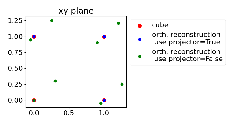
The projection allows an optimal reconstruction of the cube while when not using a projection the orthogonal condition does not allow the same reconstruction.

fig, ax_xy = plt.subplots(figsize=(7.5, 4))

ax_xy.scatter(
    xy_plane_projected_cube[:, 0],
    xy_plane_projected_cube[:, 1],
    s=70,
    c="r",
    label="cube",
)

ax_xy.scatter(
    orth_reg_use_projector_xy_plane_pred_cube[:, 0],
    orth_reg_use_projector_xy_plane_pred_cube[:, 1],
    c="b",
    label="orth. reconstruction\n use projector=True",
)

ax_xy.scatter(
    orth_reg_xy_plane_pred_cube[:, 0],
    orth_reg_xy_plane_pred_cube[:, 1],
    c="g",
    label="orth. reconstruction\n use projector=False",
)

ax_xy.set_title("xy plane")

ax_xy.legend(loc="upper left", bbox_to_anchor=(1, 1))

fig.tight_layout()
fig.show()

The three dimensional cubic structure can be seen when no projector is used (use_orthogonal_projector is False). Now we plot the prediction error.

fig, (ax_with_orth, ax_wo_orth) = plt.subplots(ncols=2, figsize=(10, 4.5), sharey=True)

ax_with_orth.scatter(
    z_scalings,
    regression_errors_for_z_scaled_square_prism_using_orthogonal_projector,
)
ax_with_orth.scatter(
    0,
    regression_error_for_xy_plane_projected_cube_using_orthogonal_projector,
)
ax_with_orth.set_title(
    "Orthogonal regression error for\n features using orthogonal projector\n "
    "(use_orthogonal_projector=True)",
    fontsize=14,
)
ax_with_orth.set_xlabel("scaling in z direction", fontsize=16)
ax_with_orth.set_ylabel("orthogonal regression error", fontsize=14)

ax_wo_orth.scatter(
    z_scalings,
    regression_errors_for_z_scaled_square_prism_zero_padded,
    label="z-scaled square prism",
)
ax_wo_orth.scatter(
    0,
    regression_error_for_xy_plane_projected_cube_zero_padded,
    label="xy_plane_projected_cube",
)
ax_wo_orth.set_title(
    "Orthogonal regression error for\n zero padded features\n "
    "(use_orthogonal_projector=False) ",
    fontsize=14,
)
ax_wo_orth.set_xlabel("scaling in z direction")
fig.tight_layout()
ax_wo_orth.legend(loc="lower left", title="Regression error", fontsize=12)

fig.show()

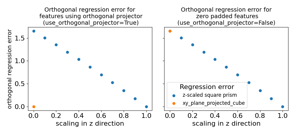
It can be seen that if use_orthogonal_projector is set to True, the regression error of xy_plane_projected_cube has an abrupt jump in contrast to retaining the third dimension with 0 values. When use_orthogonal_projector is set to False this non-analytic behavior is not present, since it uses the padding solution. Both methods have valid reasons to be applied and have their advantages and disadvantages depending on the use case.