Note
Go to the end to download the full example code.
Probabilistic Analysis of Molecular Motifs (PAMM)#
Probabilistic analysis of molecular motifs (PAMM) is a method identifying molecular patterns based on an analysis of the probability distribution of fragments observed in an atomistic simulation. With the help of sparse KDE, it can be easily conducted.
Here we define some functions to help us. quick_shift_refinement is used to refine the clusters generated by QuickShift by merging outlier clusters into their nearest neighbours. generate_probability_model is to interpret the quick shift results into a probability model. cluster_distribution_3D is to plot the probability model of the H-bond motif.
from typing import Callable, Union

import matplotlib.pyplot as plt
import numpy as np
from scipy.special import logsumexp

from skmatter.clustering import QuickShift
from skmatter.datasets import load_hbond_dataset
from skmatter.feature_selection import FPS
from skmatter.metrics import periodic_pairwise_euclidean_distances
from skmatter.neighbors import SparseKDE
from skmatter.neighbors._sparsekde import _covariance
from skmatter.utils import oas
def quick_shift_refinement(
    X: np.ndarray,
    cluster_centers_idx: np.ndarray,
    labels: np.ndarray,
    probs: np.ndarray,
    metric: Callable = periodic_pairwise_euclidean_distances,
    metric_params: Union[dict, None] = None,
    thrpcl: float = 0.0,
):
    """
    Parameters
    ----------
    X : np.ndarray
        Input data for fitting of quick shift
    cluster_centers_idx : np.ndarray
        Index of the cluster centers in `X`
    labels : np.ndarray
        Labels of the input data, generated by `QuickShift`
    probs : numpy.ndarray
        Probability density of the input data
    metric : Callable, default=pairwise_euclidean_distances
        The metric to use.
    metric_params : dict, default=None
        Additional parameters to be passed to the use of
        metric.  i.e. the cell dimension for `periodic_euclidean`
        {'cell': [2, 2]}
    thrpcl : float, default=0.0
    Clusters with a pk lower than this value are merged with the nearest cluster.
    """
    if metric_params is not None:
        cell = metric_params["cell_length"]
        if len(cell) != X.shape[1]:
            raise ValueError("Cell dimension does not match the data dimension.")
    else:
        cell = None

    normpks = logsumexp(probs)
    nk = len(cluster_centers_idx)
    to_merge = np.full(nk, False)

    for k in range(nk):
        dummd1 = np.exp(logsumexp(probs[labels == cluster_centers_idx[k]]) - normpks)
        to_merge[k] = dummd1 > thrpcl
    # merge the outliers
    for i in range(nk):
        if not to_merge[k]:
            continue
        dummd1yi1 = cluster_centers_idx[i]
        dummd1 = np.inf
        for j in range(nk):
            if to_merge[k]:
                continue
            dummd2 = metric(X[labels[dummd1yi1]], X[labels[j]], cell=cell)
            if dummd2 < dummd1:
                dummd1 = dummd2
                cluster_centers_idx[i] = j
        labels[labels == dummd1yi1] = cluster_centers_idx[i]
    if sum(to_merge) > 0:
        cluster_centers_idx = np.concatenate(
            np.argwhere(labels == np.arange(len(labels)))
        )
        nk = len(cluster_centers_idx)
        for i in range(nk):
            dummd1yi1 = cluster_centers_idx[i]
            cluster_centers_idx[i] = np.argmax(
                np.ma.array(probs, mask=labels != cluster_centers_idx[i])
            )
            labels[labels == dummd1yi1] = cluster_centers_idx[i]

    return cluster_centers_idx, labels
def generate_probability_model(
    cluster_center_idx: np.ndarray,
    labels: np.ndarray,
    X: np.ndarray,
    descriptors: np.ndarray,
    descriptor_labels: np.ndarray,
    descriptor_weights: np.ndarray,
    probs: np.ndarray,
    cell: np.ndarray = None,
):
    """
    Generates a probability model based on the given inputs.

    Parameters
    ----------
    cluster_center_idx : np.ndarray
        Index of the cluster centers in `X`
    labels : np.ndarray
        Labels of the input data, generated by `QuickShift`
    X : np.ndarray
        Input data
    descriptors : np.ndarray
        Descriptors from original data set
    descriptor_labels : np.ndarray
        Labels of the descriptors, generated by
        `skmatter.neighbors._sparsekde._NearestGridAssigner`
    descriptor_weights : np.ndarray
        Weights of the descriptors
    probs : np.ndarray
        Probability density of the input data
    cell : np.ndarray
        Cell dimension for distance metrics
    """

    def _update_cluster_cov(
        X: np.ndarray,
        k: int,
        sample_labels: np.ndarray,
        probs: np.ndarray,
        idxroot: np.ndarray,
        center_idx: np.ndarray,
    ):
        if cell is not None:
            cov = _get_lcov_clusterp(
                len(X), nsamples, X, idxroot, center_idx[k], probs, cell
            )
            if np.sum(idxroot == center_idx[k]) == 1:
                cov = _get_lcov_clusterp(
                    nsamples,
                    nsamples,
                    descriptors,
                    sample_labels,
                    center_idx[k],
                    descriptor_weights,
                    cell,
                )
                print("Warning: single point cluster!")
        else:
            cov = _get_lcov_cluster(len(X), X, idxroot, center_idx[k], probs, cell)
            if np.sum(idxroot == center_idx[k]) == 1:
                cov = _get_lcov_cluster(
                    nsamples,
                    descriptors,
                    sample_labels,
                    center_idx[k],
                    descriptor_weights,
                    cell,
                )
                print("Warning: single point cluster!")
            cov = oas(
                cov,
                logsumexp(probs[idxroot == center_idx[k]]) * nsamples,
                X.shape[1],
            )

        return cov

    def _get_lcov_cluster(
        N: int,
        x: np.ndarray,
        clroots: np.ndarray,
        idcl: int,
        probs: np.ndarray,
        cell: np.ndarray,
    ):
        ww = np.zeros(N)
        normww = logsumexp(probs[clroots == idcl])
        ww[clroots == idcl] = np.exp(probs[clroots == idcl] - normww)
        cov = _covariance(x, ww, cell)

        return cov

    def _get_lcov_clusterp(
        N: int,
        Ntot: int,
        x: np.ndarray,
        clroots: np.ndarray,
        idcl: int,
        probs: np.ndarray,
        cell: np.ndarray,
    ):
        ww = np.zeros(N)
        totnormp = logsumexp(probs)
        cov = np.zeros((x.shape[1], x.shape[1]), dtype=float)
        xx = np.zeros(x.shape, dtype=float)
        ww[clroots == idcl] = np.exp(probs[clroots == idcl] - totnormp)
        ww *= Ntot
        nlk = np.sum(ww)
        for i in range(x.shape[1]):
            xx[:, i] = x[:, i] - np.round(x[:, i] / cell[i]) * cell[i]
            r2 = (np.sum(ww * np.cos(xx[:, i])) / nlk) ** 2 + (
                np.sum(ww * np.sin(xx[:, i])) / nlk
            ) ** 2
            re2 = (nlk / (nlk - 1)) * (r2 - (1 / nlk))
            cov[i, i] = 1 / (np.sqrt(re2) * (2 - re2) / (1 - re2))

        return cov

    if cell is not None and (X.shape[1] != len(cell)):
        raise ValueError("Cell dimension does not match the data dimension.")
    nclusters = len(cluster_center_idx)
    nsamples = len(descriptors)
    dimension = X.shape[1]
    cluster_mean = np.zeros((nclusters, dimension), dtype=float)
    cluster_cov = np.zeros((nclusters, dimension, dimension), dtype=float)
    cluster_weight = np.zeros(nclusters, dtype=float)
    center_idx = np.unique(labels)
    normpks = logsumexp(probs)

    for k in range(nclusters):
        cluster_weight[k] = np.exp(logsumexp(probs[labels == center_idx[k]]) - normpks)
        cluster_cov[k] = _update_cluster_cov(
            X, k, descriptor_labels, probs, labels, center_idx
        )
    for k in range(nclusters):
        labels[labels == center_idx[k]] = k + 1

    return cluster_weight, cluster_mean, cluster_cov, labels
def cluster_distribution_3D(
    grids: np.ndarray,
    grid_weights: np.ndarray,
    grid_label_: np.ndarray = None,
    use_index: list[int] = None,
    label_text: list[str] = None,
    size_scale: float = 1e4,
    fig_size: tuple[int, int] = (12, 12),
) -> tuple[plt.Figure, plt.Axes]:
    """
    Generate a 3D scatter plot of the cluster distribution.

    Parameters
    ----------
        grids (numpy.ndarray): The array containing the grid data.
        use_index (Optional[list[int]]): The indices of the features to use for the
            scatter plot.
            If None, the first three features will be used.
        label_text (Optional[list[str]]): The labels for the x, y, and z axes.
            If None, the labels will be set to
            'Feature 0', 'Feature 1', and 'Feature 2'.
        size_scale (float): The scale factor for the size of the scatter points.
            Default is 1e4.
        fig_size (tuple[int, int]): The size of the figure. Default is (12, 12)

    Returns
    -------
        tuple[plt.Figure, plt.Axes]: A tuple containing the matplotlib
            Figure and Axes objects.
    """
    if use_index is None:
        use_index = [0, 1, 2]
    if label_text is None:
        label_text = [f"Feature {i}" for i in range(3)]

    fig, ax = plt.subplots(subplot_kw={"projection": "3d"}, figsize=fig_size, dpi=100)
    scatter = ax.scatter(
        grids[:, use_index[0]],
        grids[:, use_index[1]],
        grids[:, use_index[2]],
        c=grid_label_,
        s=grid_weights * size_scale,
    )
    legend1 = ax.legend(*scatter.legend_elements(), loc="lower left", title="Gaussian")
    ax.add_artist(legend1)
    ax.set_xlabel(label_text[0])
    ax.set_ylabel(label_text[1])
    ax.set_zlabel(label_text[2])

    return fig, ax
We first load our dataset:
hbond_data = load_hbond_dataset()
descriptors = hbond_data["descriptors"]
weights = hbond_data["weights"]
We use the FPS class to select the ngrid descriptors with the highest. It is recommended to set the number of grids as the square root of the number of descriptors. Then we do the fit of the KDE.
ngrid = int(len(descriptors) ** 0.5)
selector = FPS(initialize=26310, n_to_select=ngrid)
selector.fit(descriptors.T)
selector.selected_idx_
grids = descriptors[selector.selected_idx_]
SparseKDE(descriptors=array([[-2.30202112,  4.25360095,  2.69259933],
       [-2.01145112,  4.15748728,  2.56943865],
       [-2.13815953,  4.04815345,  3.00762119],
       ...,
       [ 2.15450524,  4.12701864,  2.66229369],
       [ 1.40706501,  4.42784213,  3.97425917],
       [ 2.1403912 ,  4.01460208,  2.64365087]], shape=(27233, 3)),
          metric=<function SparseKDE.__init__.<locals>.<lambda> at 0x7ee56133a200>,
          metric_params={'cell_length': None},
          weights=array([3.54941673e-05, 3.59453928e-05, 3.44066147e-05, ...,
       3.70670491e-05, 1.74550114e-05, 4.00939472e-05], shape=(27233,)))
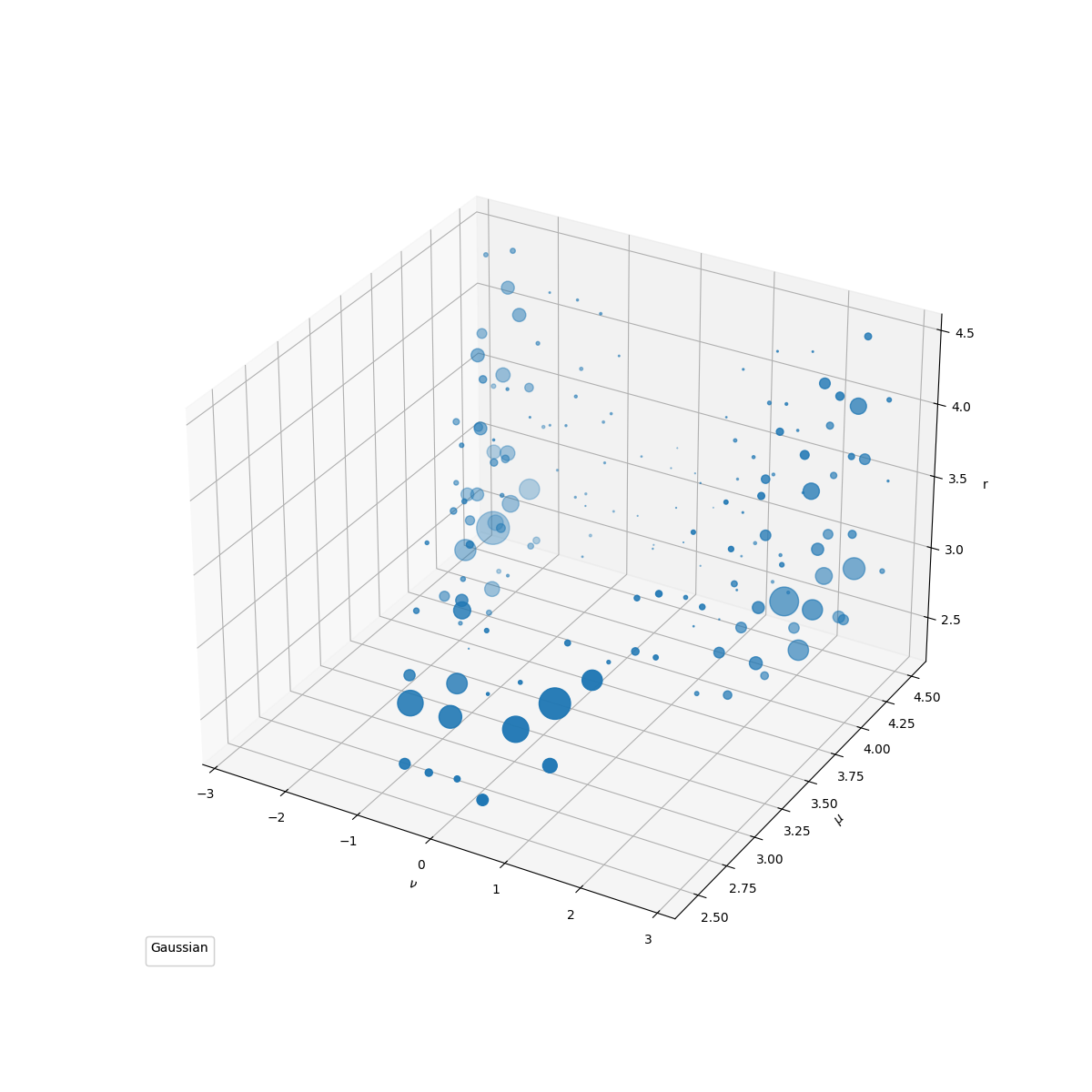
Now we visualize the distribution and the weight of clusters.
cluster_distribution_3D(
    grids, estimator._sample_weights, label_text=[r"$\nu$", r"$\mu$", r"r"]
)
/home/docs/checkouts/readthedocs.org/user_builds/scikit-matter/envs/254/lib/python3.13/site-packages/matplotlib/collections.py:1112: UserWarning: Collection without array used. Make sure to specify the values to be colormapped via the `c` argument.
  warnings.warn("Collection without array used. Make sure to "

(<Figure size 1200x1200 with 1 Axes>, <Axes3D: xlabel='$\\nu$', ylabel='$\\mu$', zlabel='r'>)
We need to estimate the probability at each grid point to do quick shift, which can further partition the set of grid points into several clusters. The resulting clusters can be interpreted as (meta-)stable states of the system.
probs = estimator.score_samples(grids)
qscuts = np.array([np.trace(cov) for cov in estimator._covariance])
clustering = QuickShift(
    qscuts**2,
    metric_params=estimator.metric_params,
)
clustering.fit(grids, samples_weight=probs)
cluster_centers_idx = clustering.cluster_centers_idx_
labels = clustering.labels_
normpks = logsumexp(probs)

cluster_centers, labels = quick_shift_refinement(
    grids,
    cluster_centers_idx,
    labels,
    probs,
    estimator.metric,
    estimator.cell,
)
Quick-Shift:   0%|          | 0/165 [00:00<?, ?it/s]
Quick-Shift: 100%|██████████| 165/165 [00:00<00:00, 24280.26it/s]
Based on the results, the Gaussian mixture model of the system can be generated:
cluster_weights, cluster_means, cluster_covs, labels = generate_probability_model(
    cluster_centers_idx,
    labels,
    grids,
    estimator.descriptors,
    estimator._sample_labels_,
    estimator.weights,
    probs,
    estimator.cell,
)
/home/docs/checkouts/readthedocs.org/user_builds/scikit-matter/envs/254/lib/python3.13/site-packages/skmatter/neighbors/_sparsekde.py:609: RuntimeWarning: invalid value encountered in divide
  cov /= 1 - sum((sample_weights / totw) ** 2)
Warning: single point cluster!
Warning: single point cluster!
Warning: single point cluster!
Warning: single point cluster!
Warning: single point cluster!
Warning: single point cluster!
Warning: single point cluster!
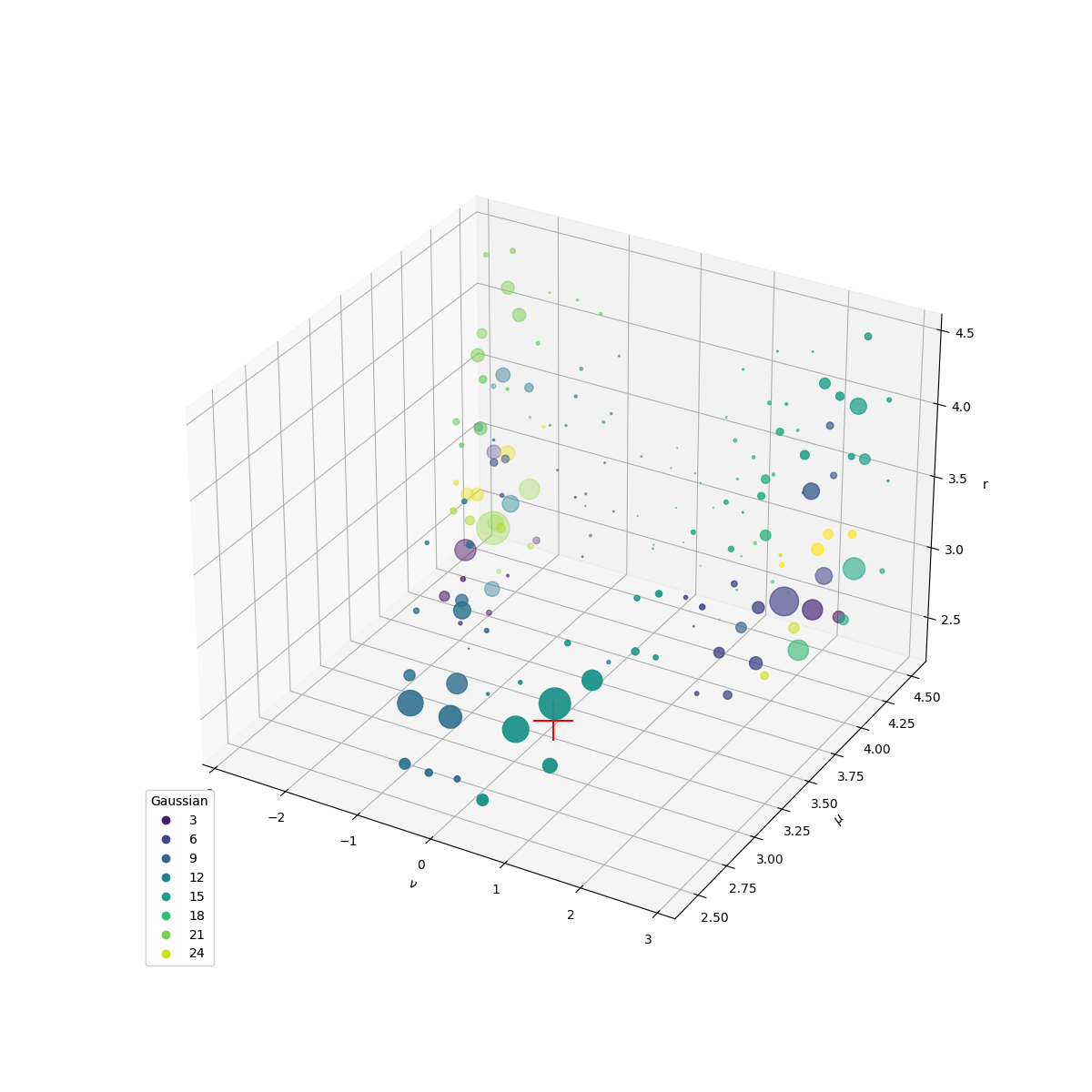
The final result shows seven (meta-)stable states of hydrogen bond. Here we also show the reference hydrogen bond descriptor. The Gaussian with the largest weight locates closest to the reference point. This result shows that, with the help of the SparseKDE and QuickShift algorithm, we can easily identify the (meta-)stable states of the system objectively and without any prior knowledge about the system.
<mpl_toolkits.mplot3d.art3d.Path3DCollection object at 0x7ee561d51090>
f"The Gaussian with the highest probability is {np.argmax(cluster_weights) + 1}"
'The Gaussian with the highest probability is 14'