Sparse KDE examples

Example for the usage of the skmatter.neighbors.SparseKDE class. This class is specifically designed for conducting pobabilistic analysis of molecular motifs (PAMM), which is quite useful for analyzing motifs like H-bonds, coordination polyhedra, and protein secondary structure.

Here we show how to use the sparse KDE model to fit the probability distribution based on sampled data and how to use PAMM to analyze the H-bond.

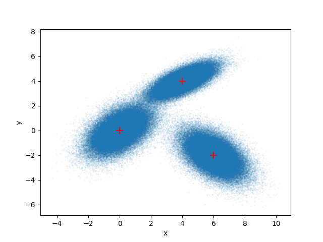
We start from a simple system, which is consist of three 2D Gaussians. Our task is to estimate the parameters of these Gaussians from our sampled data.

Here we first sample from these three Gaussians.

import time

import matplotlib.pyplot as plt
import numpy as np
from scipy.stats import gaussian_kde

from skmatter.feature_selection import FPS
from skmatter.neighbors import SparseKDE

means = np.array([[0, 0], [4, 4], [6, -2]])
covariances = np.array(
    [[[1, 0.5], [0.5, 1]], [[1, 0.5], [0.5, 0.5]], [[1, -0.5], [-0.5, 1]]]
)
N_SAMPLES = 100_000
samples = np.concatenate(
    [
        np.random.multivariate_normal(means[0], covariances[0], N_SAMPLES),
        np.random.multivariate_normal(means[1], covariances[1], N_SAMPLES),
        np.random.multivariate_normal(means[2], covariances[2], N_SAMPLES),
    ]
)

We can visualize our sample result:

fig, ax = plt.subplots()
ax.scatter(samples[:, 0], samples[:, 1], alpha=0.05, s=1)
ax.scatter(means[:, 0], means[:, 1], marker="+", color="red", s=100)
ax.set_xlabel("x")
ax.set_ylabel("y")
plt.show()

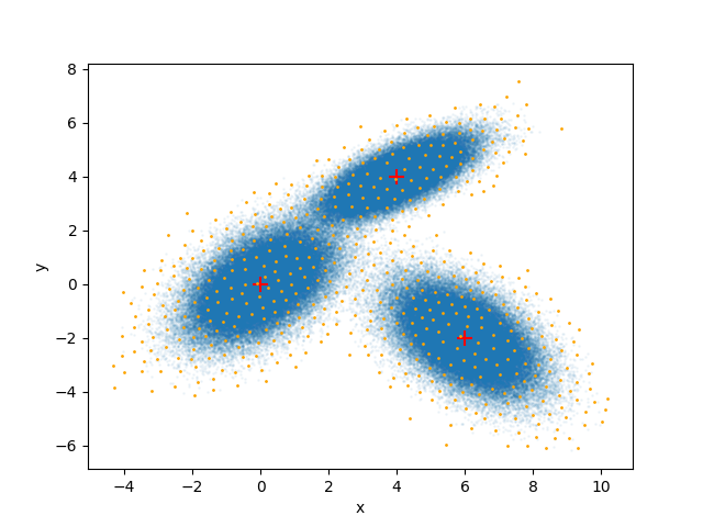
Sparse KDE requires a discretization of the sample space. Here, we use the FPS method to generate grid points in the sample space:

start1 = time.time()
selector = FPS(n_to_select=int(np.sqrt(3 * N_SAMPLES)))
grids = selector.fit_transform(samples.T).T
end1 = time.time()
fig, ax = plt.subplots()
ax.scatter(samples[:, 0], samples[:, 1], alpha=0.05, s=1)
ax.scatter(means[:, 0], means[:, 1], marker="+", color="red", s=100)
ax.scatter(grids[:, 0], grids[:, 1], color="orange", s=1)
ax.set_xlabel("x")
ax.set_ylabel("y")
plt.show()

Now we can do sparse KDE (usually takes tens of seconds):

start2 = time.time()
estimator = SparseKDE(samples, None, fpoints=0.5)
estimator.fit(grids)
end2 = time.time()

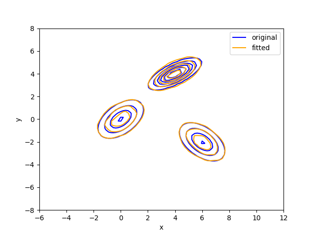
We can have a comparison with the original sampling result by plotting them.

For the convenience, we create a class for the Gaussian mixture model to help us plot the result.

class GaussianMixtureModel:
    def __init__(
        self,
        weights: np.ndarray,
        means: np.ndarray,
        covariances: np.ndarray,
        period: np.ndarray = None,
    ):
        self.weights = weights
        self.means = means
        self.covariances = covariances
        self.period = period
        self.dimension = self.means.shape[1]
        self.cov_inv = np.linalg.inv(self.covariances)
        self.cov_det = np.linalg.det(self.covariances)
        self.norm = 1 / np.sqrt((2 * np.pi) ** self.dimension * self.cov_det)

    def __call__(self, x: np.ndarray, i: int = None):
        if len(x.shape) == 1:
            x = x[np.newaxis, :]
        if self.period is not None:
            xij = np.zeros(self.means.shape)
            xij = rij(self.period, xij, x)
        else:
            xij = x - self.means
        p = (
            self.weights
            * self.norm
            * np.exp(
                -0.5 * (xij[:, np.newaxis, :] @ self.cov_inv @ xij[:, :, np.newaxis])
            ).reshape(-1)
        )
        sum_p = np.sum(p)
        if i is None:
            return sum_p

        return np.sum(p[i]) / sum_p

def rij(period: np.ndarray, xi: np.ndarray, xj: np.ndarray) -> np.ndarray:
    """Get the position vectors between two points. PBC are taken into account."""
    xij = xi - xj
    if period is not None:
        xij -= np.round(xij / period) * period

    return xij

The original model that we want to fit:

original_model = GaussianMixtureModel(np.full(3, 1 / 3), means, covariances)
# The fitted model:
fitted_model = GaussianMixtureModel(
    estimator._sample_weights, estimator._grids, estimator.bandwidth_
)

# To plot the probability density contour, we need to create a grid of points:
x, y = np.meshgrid(np.linspace(-6, 12, 100), np.linspace(-8, 8))
points = np.concatenate(np.stack([x, y], axis=-1))
probs = np.array([original_model(point) for point in points])
fitted_probs = np.array([fitted_model(point) for point in points])

fig, ax = plt.subplots()
ct1 = ax.contour(x, y, probs.reshape(x.shape), colors="blue")
ct2 = ax.contour(x, y, fitted_probs.reshape(x.shape), colors="orange")
h1, _ = ct1.legend_elements()
h2, _ = ct2.legend_elements()
ax.legend(
    [h1[0], h2[0]],
    ["original", "fitted"],
)
ax.set_xlabel("x")
ax.set_ylabel("y")
plt.show()

The performance of the probability density estimation can be characterized by the Mean Integrated Squared Error (MISE), which is defined as: \(\text{MISE}=\text{E}[\int (\hat{P}(\textbf{x})-P(\textbf{x}))^2 d\textbf{x}]\)

RMSE = np.sum((probs - fitted_probs) ** 2 * (x[0][1] - x[0][0]) * (y[1][0] - y[0][0]))
print(f"Time sparse-kde: {end2 - start2} s")
print(f"RMSE = {RMSE:.2e}")

Time sparse-kde: 44.906388998031616 s
RMSE = 7.22e-04

We can compare the result with the KDE class from scipy. (Usually takes several minutes to run)

data = np.vstack([x.ravel(), y.ravel()])
start = time.time()
kde = gaussian_kde(samples.T)
sklearn_probs = kde(data).T
end = time.time()
print(f"Time scipy: {end - start} s")
RMSE_kde = np.sum(
    (probs - sklearn_probs) ** 2 * (x[0][1] - x[0][0]) * (y[1][0] - y[0][0])
)
print(f"RMSE_kde = {RMSE_kde:.2e}")

Time scipy: 16.33100938796997 s
RMSE_kde = 8.85e-04

We can see that the fitted model can perfectly capture the original one. Even though we have not specified the number of the Gaussians, it can still perform well. This allows us to fit distributions of the data automatically at a comparable quality within a much shorter time than scipy.